Topology Optimization Manufacturability
A concern in topology optimization is that the design concepts developed are very often not manufacturable. Another problem is that the solution of a topology optimization problem can be mesh dependent, if no appropriate measure is taken.
OptiStruct offers a number of different methods to account for manufacturability when performing topology optimization:
Member Size Control
Allows you some control over the member size in the final topology and the resulting degree of simplicity of the final design.
| (1) | (2) | (3) | (4) | (5) | (6) | (7) | (8) | (9) | (10) |
|---|---|---|---|---|---|---|---|---|---|
| DOPTPR | MINDIM | VALUE |
| (1) | (2) | (3) | (4) | (5) | (6) | (7) | (8) | (9) | (10) |
|---|---|---|---|---|---|---|---|---|---|
| DTPL | ID | PTYPE | PID1 | PID2 | PID3 | PID4 | PID5 | PID6 | |
| PID7 | etc | etc | etc | ||||||
| MEMBSIZ | MINDIM | MAXDIM | MINGAP |
Here, both the preferred minimum, MINDIM, and the maximum, MAXDIM, diameter of members may be defined on the MEMBSIZ continuation line. Member size dimensions can be defined differently for each DTPL in this way. MINGAP defines the minimum spacing between structural members formed. It is only used in conjunction with MAXDIM. Usage of MAXDIM implies that the a MINGAP constraint of the same value as MAXDIM is applied. Therefore, for MINGAP to be effective, it should be greater than MAXDIM.
Minimum Member Size Control
Although minimum member size control penalizes the formation of small members, results that contain members significantly under the specified minimum member size can still be obtained.
This is because a small member in the structure can be very important to the load transmission and may not be removed by penalization. Minimum member size control functions more as a quality control than a quantity control.
A discrete solution is achieved in two iterative steps. The first step converges to a solution with a large number of semi-dense elements. The second step tries to refine this solution to a solution with fully dense members. Each step consists of a number of iterations. The first step consists of two entire convergence phases - the first run with the initial discreteness values (defined by DISCRETE and DISCRT1D parameters on the DOPTPRM Bulk Data Entry), followed by a run with the discreteness values increased by 1.0. This procedure is implemented in order to achieve a solution with clearly defined members. If this step could not create a solution with clearly defined members, the preferred minimum member size will not be preserved in the second step. In which case, you need to increase the discreteness parameters and/or reduce the convergence tolerance (defined by the OBJTOL parameter on the DOPTPRM Bulk Data Entry) to improve the solution of the first phase. The default discreteness is set to 1.0 for 1D elements, plates and shells, and 2.0 for 3D solids.
In general, once MINDIM is activated, checkerboarding is controlled by the methods applied for this feature, eliminating the need for the CHECKER parameter. In rare circumstances, checkerboards may still be introduced in the second phase described above for 3D solids. If this happens, an additional checkerboard control algorithm can be activated with the MMCHECK parameter. (The CHECKER and MMCHECK parameters are defined using the DOPTPRM Bulk Data Entry).
The use of this card will assure a checkerboard-free solution, although with the undesired side effect of achieving a solution that involves a large number of semi-dense elements, similar to the result of setting CHECKER equal to 1. Therefore, use this card only when it is necessary.
It is recommended that MINDIM be at least 3 times, and no greater than 12 times, the average element size for all elements referenced by that DTPL (or all designable elements when defined on DOPTPRM). The average element size for 2D elements is calculated as the average of the square root of the area of the elements, and for 3D elements, as the average of the cubic root of the volume of the elements.
This recommendation is enforced when combined with other manufacturing constraints, and if the defined MINDIM is less than this value, it will be reset to a default value equal to 3 times the average element size. Similarly, if the defined MINDIM is larger than 12 times the average element size, it will be reset to a value equal to 12 times the average element size. This limit has been set to trim memory requirements that can become too large as a result of having to keep track of a much larger number of elements needed to satisfy the MINDIM constraint. In structures where the mesh is aligned with the draw or extrusion direction, setting MTYP as ALIGN on the MESH continuation line of the DTPL card may circumvent this constraint.
MINDIM can be smaller than the mesh size. When a value smaller than the mesh size is applied, the effect is similar to checkerboard control but with the 3-phase convergence phases process and possibly a more discrete result. Minimum member size control has a 3-phase iterative process where the final phase targets the removal of the semi-dense element layer. If manufacturing constraints are applied, minimum member size control is always activated. However, the final iterative phase will not target the removal of semi-dense elements as this may have an adverse effect on manufacturing constraint preservation.
- Michell-truss Example
- MBB-Beam Example
- Arch Example
- 3D Bridge Model Example
Maximum Member Size Control
Penalizes the formation of large members. The control is not directional, meaning that if the thickness of a member is less than MAXDIM in any direction, this constraint is satisfied. This reflects the need to control the rib thickness of casting parts.
MAXDIM must be at least twice MINDIM, and hence the minimum mesh requirement is that MAXDIM has to be at least 6 times the average element size for all elements referenced by that DTPL. This constraint is strongly enforced and an error termination will occur when this criteria is not met. In addition, MAXDIM should be less than half the width of the thinnest part of the design region.
Based on the constraints mentioned above, a fine mesh is required to achieve good results with this manufacturing constraint.
It is to be noted that use of the maximum member size control induces further restriction of the feasible design space and should therefore only be used when it is truly desirable. Also, this feature is a new research development, and the techniques are still undergoing improvement. An undesired side effect that has been noticed for some examples is that it might result in more intermediate density in the final solution. Therefore, it is recommended that this feature be used sparingly until the technology becomes more robust.
While MAXDIM also enforces a spacing of members of the same dimension, the maximum reachable volume fraction is 0.5. For problems involving constraints on structural responses, this could interfere with constraint satisfaction. It is strongly recommended that the behavior of the design problem be studied without MAXDIM first in order to determine if the use of MAXDIM would be advantageous, and if the target volume allows for it to be applied.
The following examples demonstrate the impact of maximum member size control to the design outcome.
Example: Engine Bracket
Example: Steering Wheel Bracket
Draw Direction Constraints
In the casting process, cavities that are not open and lined up with the sliding direction of the die are not feasible. Designs obtained by topology optimization often contain cavities that are not viable for casting.
Transformation of such a design proposal to a manufacturable design could be extremely difficult, if not impossible. In some cases where this transformation is made, the likelihood of severely affecting the design optimality is high.
OptiStruct allows you to impose draw direction constraints so that the topology determined will allow the die to slide in a given direction. These constraints are defined using the DTPL card. Different constraints can be applied to different structural parts, specified by PSOLID IDs. There are two DRAW options available. The option SINGLE assumes that a single die will be used and it slides in the given drawing direction. The bottom surface of the considered casting part is the predefined contra part for the die. The option SPLIT implies that two dies splitting apart in the given draw direction will be used to cast the part described in this DTPL card. The splitting surface of the two dies is optimized during the optimization process.
It is often a requirement of certain designs that no through - holes exist. These holes can be prevented from forming in the direction of the draw through use of the NO HOLE option. This parameter is also defined on the DTPL card. With NO HOLE, the topology can only evolve gradually from the boundary one layer at a time, and in certain cases, it may take several iterations to remove one layer.
Available with the SINGLE draw option is a stamping or sheet metal manufacturing constraint. This option forces the evolution of 3D shell interpretable structure from a 3D design domain. This allows the design of 2D shell or stamped parts from a 3D design domain allowing greater design flexibility. The STAMP option is also specified on the DTPL card along with a thickness value that represents the desired thickness of the resulting shell or stamped part.
A casting may contain a non-designable region in addition to a designable region. These non-designable regions must be defined as obstacles for the casting process on the same DTPL card. This preserves the casting feasibility of the final structure.
Also, there is a default minimum member size for use with draw direction constraints. This is determined internally to be three times the average mesh size of the relevant components. Therefore, the mesh density of the model and the target volume fraction should be chosen so that enough material is available to fill members of the default minimum size. You can specify a desired minimum member size for each design part defined by a DTPL card. This value must be larger than the default value or else it will be replaced by the default value.
Example: Beam under Torsion
As expected, the result without manufacturing constraints is a tube-like structure that is indeed the optimal topology for torsion load. However, this design does not permit the sliding of the die in the Z direction. The result that allows the sliding of the die for casting is not very intuitive, it forms a periodical X pattern to cross the pair of twist loads until they reach the supported end. Significantly more material at the crossing point reflects the doubled shear force at this point. Compared to an upward facing C channel solution, the cross pattern has the advantage that the stress is periodical in every X cell, thus eliminating higher order influence of the span of the beam for any solution that has system level bending action.
Example: Engine Bracket
Example: Compressor Mounting Bracket
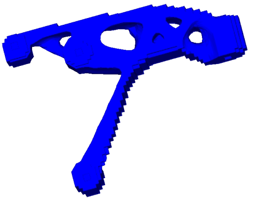
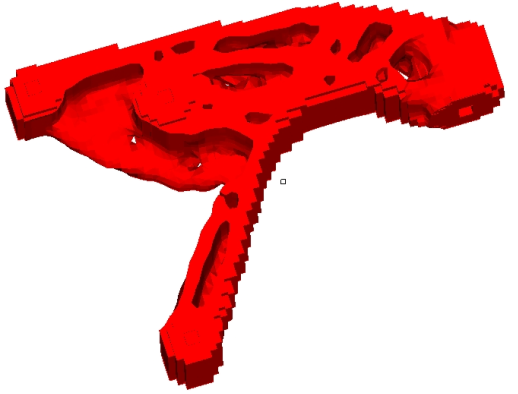
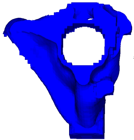
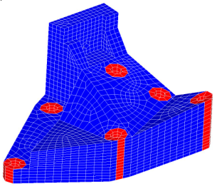
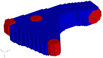
A topology optimization is run on a compressor mounting bracket, and the effects of the NO HOLE manufacturing constraint will be showcased. The finite element model is shown in Figure 12. Regions in red indicate non-design space and the region in blue indicates design space. Four different loading conditions were considered representing operating conditions, and the model was built up with approximately 90,000 elements. The design problem was formulated to minimize the compliance as the objective function, with a constraint on the design volume fraction.
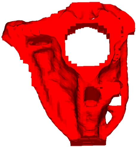
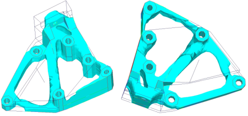
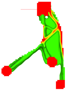
Figure 13 shows the design proposal for the compressor mounting bracket without the use of the NO HOLE manufacturing constraint. As seen in the image, the design contains through-holes.
Example: Automotive Bracket
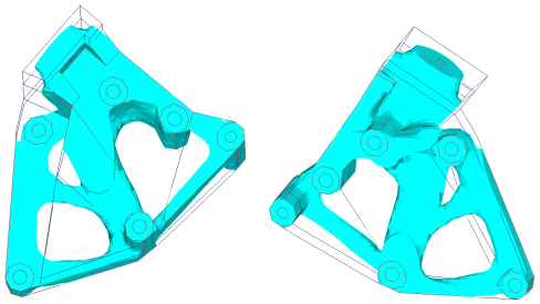
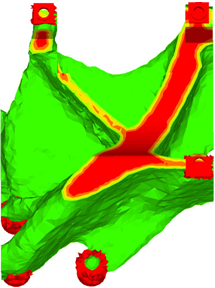
The bracket here was designed incorporating the NO HOLE constraint along with the STAMP constraint. The goal of the study was to generate a design proposal without any through-holes, while at the same time being interpretable as a sheet metal design. The STAMP constraint here forces the formation of a 3D shell interpretable structure representing a sheet metal design. Four subcases representing four different loading conditions were considered and the model was comprised of approximately 20,000 elements. The optimization problem was formulated to minimize the weighted compliance (one compliance value per subcase) for a constrained design volume fraction. This essentially results in evolving the stiffest design for a given amount of material.
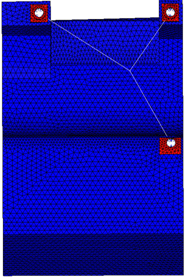
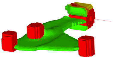
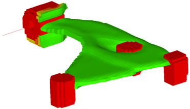
Figure 15 represents the finite element model of the design and non-design spaces of the bracket. The regions in red are the non-design regions and the region in blue is the design space.
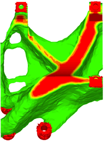
Figure 16 is the design proposal without the consideration of the STAMP and NO HOLE manufacturing requirements. While it is possible to cast such a design, stamping such a part is not feasible.
Extrusion Constraints
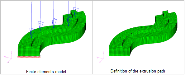
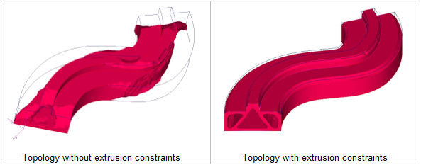
By using extrusion manufacturing constraints in topology optimization, constant cross-section designs can be attained for solid models - regardless of the initial mesh, boundary conditions or loads.
In some cases, it is desirable to produce a design characterized by a constant cross-section along a given path, particularly for parts manufactured through an extrusion process.
Extrusion constraints can also be used for the conceptual design study of structures that do not specifically need to be manufactured using an extrusion procedure. Those requirements can be regarded as specific geometric constraints and can be used for any design that desires such characteristics. For instance, it might be desirable to have ribs going through the entire depth of a solid domain.
As with other manufacturing constraints, extrusion constraints can be applied on a component level, and can be defined in conjunction with Minimum Member Size Control using the DTPL card.
Problem Setup

Define the Extrusion Path

In the example above, four grids are used to define the extrusion path (left figure), where the path computed by OptiStruct is inaccurate. To obtain a more accurate approximation, more grids are included in the extrusion path (right figure).
For twisted cross-sections, a secondary extrusion path needs to be defined in a similar manner through the EPATH2 field.
Example: Curved Beam
Example: Stair Shaped Structure
Example: Extrusion Constraints
Pattern Repetition
A technique where different structural components can be linked together so as to produce similar topological layouts.
To achieve this, a main DTPL card needs to be defined, followed by any number of secondary DTPL cards which reference the main. The main and secondary components are related to each other through local coordinate systems, which are required, and through scaling factors, which are optional.
Other manufacturing constraints, such as minimum or maximum member size, draw direction constraints or extrusion constraints, can be applied to the main DTPL card. These constraints will then automatically be applied to the secondary DTPL card(s).
- Create a main DTPL card.
- Apply other manufacturing constraints as needed.
- Define the local coordinate system associated to the main DTPL card.
- Create a secondary DTPL card.
- Define the local coordinate systems associated to the secondary DTPL card.
- Apply scaling factors as needed.
- Repeat steps 4-6 for any number of secondary DTPL cards.
Local Coordinates Systems
- CAID
- Defines the anchor point for the local coordinates system.
- CFID
- Defines the direction of the X-axis.
- CSID
- Defines the XY plane and indicates the positive sense of the Y-axis.
- CTID
- Indicates the positive sense of the Z-axis.

Scaling Factors

Pattern Repetition with Draw Direction Constraints
Draw direction constraints can be applied simultaneously with pattern repetition. To achieve this, simply define the draw direction for the main DTPL card, and the draw direction for the secondary(ies) will automatically be generated based on the local coordinate system.
Even if some components are not naturally identical, the optimized design for each component will still satisfy the draw direction constraints. In particular, if different components contain different obstacles, the combination of all obstacles will always be considered.
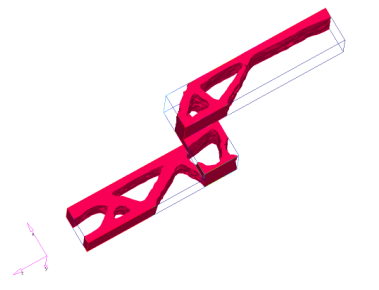
Pattern Repetition with Extrusion Constraints
Extrusion constraints can also be used in conjunction with pattern repetition. This allows for creating parts which have identical cross-sections. The components do not need to be identical in a three-dimensional sense; each part can have its own extrusion path.
If the components have different extrusion paths, these paths have to be defined explicitly on each DTPL card. However, if the components have identical extrusion paths, the paths for the secondary(ies) will automatically be computed based on the main's extrusion path.
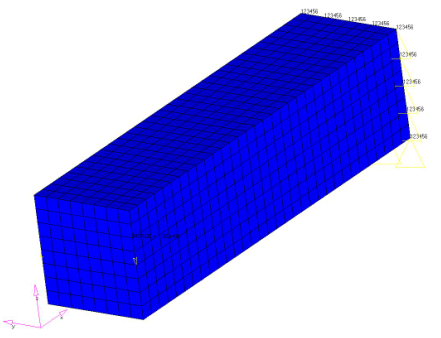
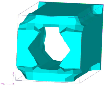
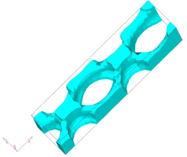
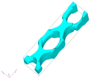
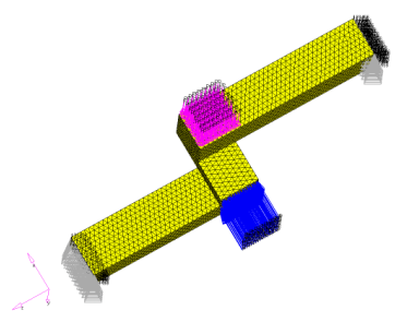
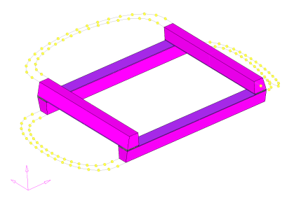
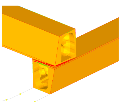
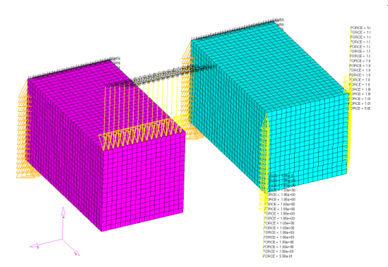
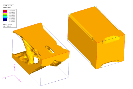
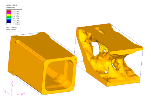
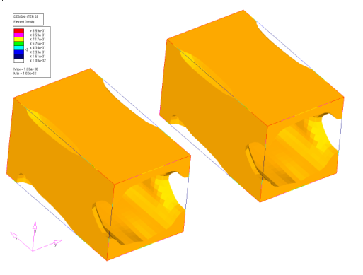
Example: Block Models
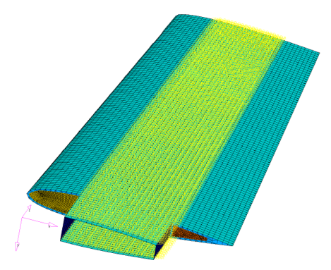
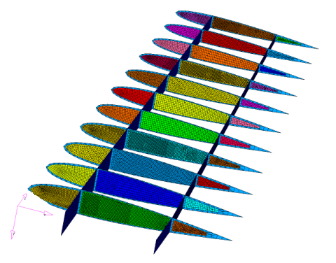
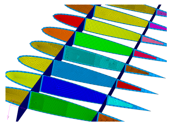
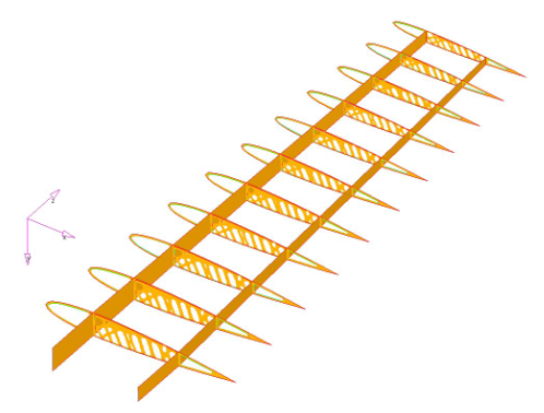
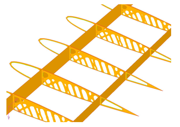
Example: Simplified Wing Model
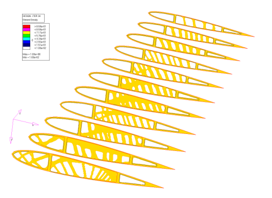
Pattern Grouping
Pattern grouping is a feature that allows you to define a single part of the domain that should be designed in a certain pattern.
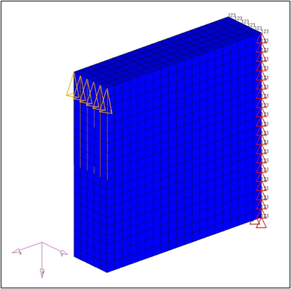
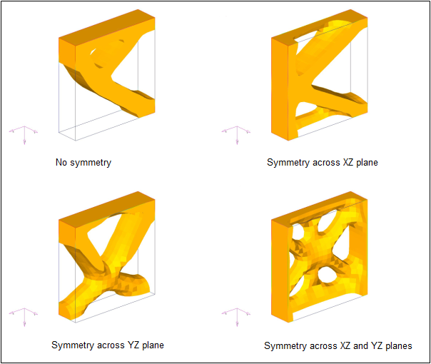
Planar Symmetry
It is often desirable to produce a design that has symmetry. Unfortunately, even if the design space and boundary conditions are symmetric, conventional topology optimization methods do not guarantee a perfectly symmetric design.
By using symmetry constraints in topology optimization, symmetric designs can be attained regardless of the initial mesh, boundary conditions, or loads. Symmetry can be enforced across one plane, two orthogonal planes, or three orthogonal planes. A symmetric mesh is not necessary, as OptiStruct will create variables that are very close to identical across the plane(s) of symmetry.


Uniform Element Density
Pattern grouping also provides the possibility to request a uniform element density throughout selected components.
This pattern group ensures that all elements of selected components maintain the same element density with respect to one another.
Cyclical Symmetry
Cyclical symmetry can also be defined through the use of pattern grouping.
With cyclical pattern grouping, the design is repeated about a central axis a number of times determined by you. Furthermore, the cyclical repetitions can be symmetric within themselves. If that option is selected, OptiStruct will force each wedge to be symmetric about its centerline.


Draw Constraints
Draw direction constraints can be combined with pattern grouping.

The same reasoning applies for two-plane and three-plane symmetries, as well as for cyclical symmetry.
Caution should be used in order to achieve manufacturable designs. With cyclical symmetry, for instance, the draw direction should be parallel to the axis of symmetry.
Extrusion Constraints
Currently extrusion constraints cannot be used simultaneously with pattern grouping.
Example: Solid Block
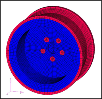
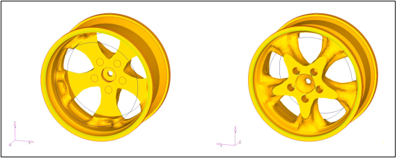
Example: Car Wheel Model