Evaluate squeak and rattle issues when exposed to thermal loading.
A typical challenge faced in the automotive industry is how does the vehicle
interior perform under driving conditions while the vehicle has been parked in the
sun for many hours?
To answer this question, vibration loads responses (Dynamics)
need to be superposed to the temperature effect on parts (Thermal Expansion – Static),
gaps are reduced for example. In this workflow, the user will evaluate the squeak and
rattle issues in a dynamic condition where the vehicle, in this case, a parked under
sunlight with a spike in internal temperature (Static loadcase). Later the car is
driven, which is exposed to Dynamic Loading. Below is the illustration of the Driving
Vehicle exposed to the Thermal Effects (Combined Loading) workflow.
The objectives of
this tutorial are:
Prepare the FE model for analyzing squeak and rattle issues.
Apply a static load of amplitude -5.55 to the certain node(s) on Lower
Control Panel component. This simulates a touch point scenario.
Run analysis and post-process the results.
For this tutorial, use a new model and prepare the model analysis setup.
For this workflow, refer the following sections from Detailed Risk and Root Cause Analysis:
Import a model with Dynamic Event loadcase. For this workflow, you can use the
model with solver deck created in the Detailed Risk and Root Cause Analysis usecase along
with the Dynamic Loadcase. Choose the workflow according to your need and refer to
sections mentioned above for the procedures.
For this tutorial, you will use
the solver deck exported from the Detailed Risk and Root Cause Analysis usecase. Once
you import the Dynamic Loadcase solver deck, you can proceed with Thermal (Static)
Loadcase setup.
Define Thermal Loadcase
In this step, you will create a thermal loadcase.
From the Setup group, select drop down arrow next to Dynamic > Thermal Event.
Figure 1.
A guide bar opens.
Select the nodes on the top surface of the IP Substrate and Dashboard Panel
components.
Figure 2.
In the guide bar, enter 90 for the
temperature value.
Click .
The Thermal loadcase with the load collectors and other entities
required for the simulation is created. Respective load collectors get created
and are assigned to the loadstep.
A user message opens.Figure 3.
Click OK.
Define Constraint
In this step, you will define model constraints.
In the Setup ribbon, select Static Event > Setup Constraints.
Figure 4.
A guide bar opens.
In the graphics area, select the node shown in Figure 5.
Figure 5.
In the microdialog, select
SnRD_STATIC_Temperature_1 for the Loadstep
option.
In the microdialog, select all degrees of
freedom.
Figure 6.
Click .
The Static loadcase with the load collectors and other entities required
for the simulation is created. Respective load collectors get created and are
assigned to the loadstep.
Import Model and Results File
In this step, you will use SnRD Post to post process the
results.
Open HyperView.
From the menu bar, click File > Load > Preferences File.
The Preferences dialog opens.
From the Preferences dialog, select Squeak
& Rattle and click Load.
The SnRD menu is created in the HyperView client.
Select SnRD > SnRD-Post.
The SnRD Post Processing tool opens.Figure 7.
Using the file browse option , select the OptiStruct
solver file which was exported in Export OptiStruct Solver File for Model File.
Note: Pre output CSV file containing the E-Lines definition is sourced automatically.
Click .
A file browser dialog opens.
Select the Tutorial_IP_SNR_Model.pch and
Tutorial_IP_SNR_Model.h3d files from the tutorials
folder.
A working status dialog opens while the H3D data is read.
Enable the checkbox against the subcase in the Subcase selection table.
Click in the Save Session File
entry field.
Browse and select the required folder where the post processing session and
data will be stored.
Figure 8.
Post Processing
In this step, you will perform a Full Analysis to understand the squeak and rattle risks in the model.
In the Post Processing tab, define the following
parameters.
For Analysis Type, select Rattle &
Squeak.
For Line(s) to Evaluate, select All.
For % statistical evaluation, enter 0.
For Session Type, select Full Analysis.
Click Execute.
Note: Execution of Full Analysis will take a considerable
amount of time to chart histograms and plot contours based on the machine's
performance.
An execution success message opens.Figure 9.
Click Close.
Full analysis creates 22 pages containing all the details. The summary for Dynamic
Loadcase Rattle analysis can be found on Page one.Figure 10. Rattle Summary Dynamic
Summary for Dynamic Loadcase Squeak analysis can be found on Page eight.Figure 11. Squeak Summary Dynamic
Summary for Thermal Loadcase Rattle analysis can be found on Page 12.Figure 12. Rattle Summary Thermal
Summary for Thermal Loadcase Squeak analysis can be found on Page 19.Figure 13. Squeak Summary Thermal
Combined Loading
In this step, you will perform a Combined Loading study to understand the thermal
effects on the squeak and rattle issues under Dynamic Loading condition.
Select the Combined Loadings tab.
Figure 14.
From the Loading Type 1 drop-down list, select dynamic
loadcase.
The Affects Gap for loading type 1 is disabled.
Click Summary Analysis.
Summary Analysis creates a summary for the combined loading effects on all
E-Lines.
Click Combine Results.
The Combined Loading summary page is created.Figure 15.
Considering the 19513009 E-Line, the following
observation that can be made for the study: The Relative Displacements has
increased from 1.83 mm to 2.09 mm under thermal effect.
Enable the Affects Gap checkbox from the Loading Type 2
list.
Select 19513009 from the E-Line(s) Selection list.
Click Full Analysis.
Click Combine Results.
The combined effect on the selected interface is plotted in the results
page.Figure 16.
The following changes can be observed from the plots:
NewGap_Nominal_LC5_R2_Z and
NewGap_Tolerance_LC5_R2_Z are introduced in the
analysis. These are the changes in gap and tolerance due to thermal
effects.
The relative displacement has reduced from 2.09 mm to 1.83 mm. This
analysis states that the thermal effects has reduced the relative
displacement, in turn leading to reduced rattle noise.
 Figure 1. A guide bar opens.
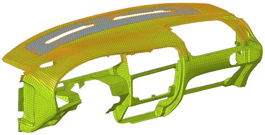 Figure 2.
  .
The Thermal loadcase with the load collectors and other entities required for the simulation is created. Respective load collectors get created and are assigned to the loadstep.A user message opens.
.
The Thermal loadcase with the load collectors and other entities required for the simulation is created. Respective load collectors get created and are assigned to the loadstep.A user message opens.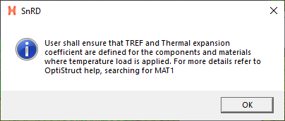 Figure 3.
  Figure 4. A guide bar opens.
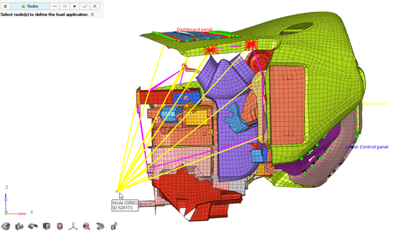 Figure 5.
  Figure 6.
 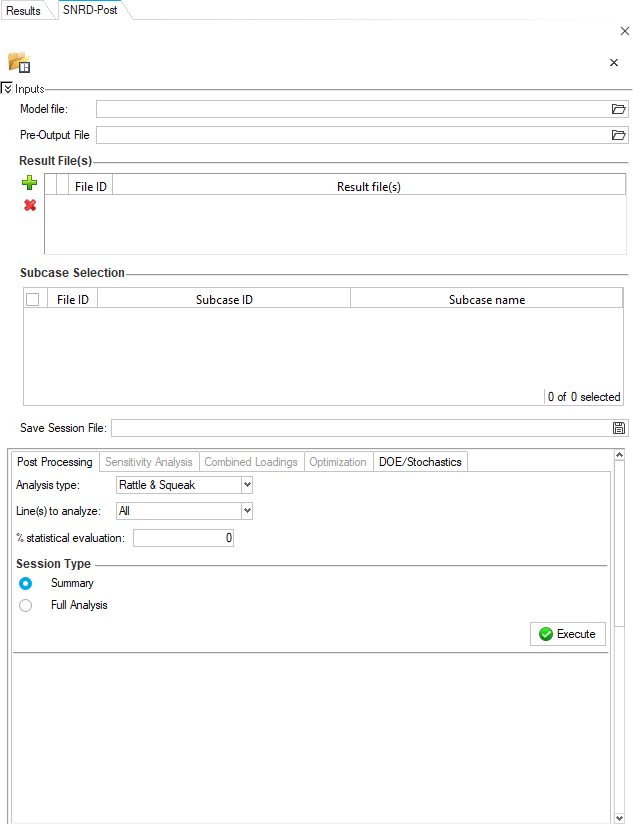 Figure 7.
  , select the OptiStruct
solver file which was exported in Export OptiStruct Solver File for Model File.
Note: Pre output CSV file containing the E-Lines definition is sourced automatically.
, select the OptiStruct
solver file which was exported in Export OptiStruct Solver File for Model File.
Note: Pre output CSV file containing the E-Lines definition is sourced automatically. .
A file browser dialog opens.
.
A file browser dialog opens. in the Save Session File
entry field.
in the Save Session File
entry field.
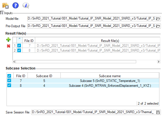 Figure 8.
 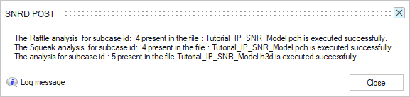 Figure 9.
 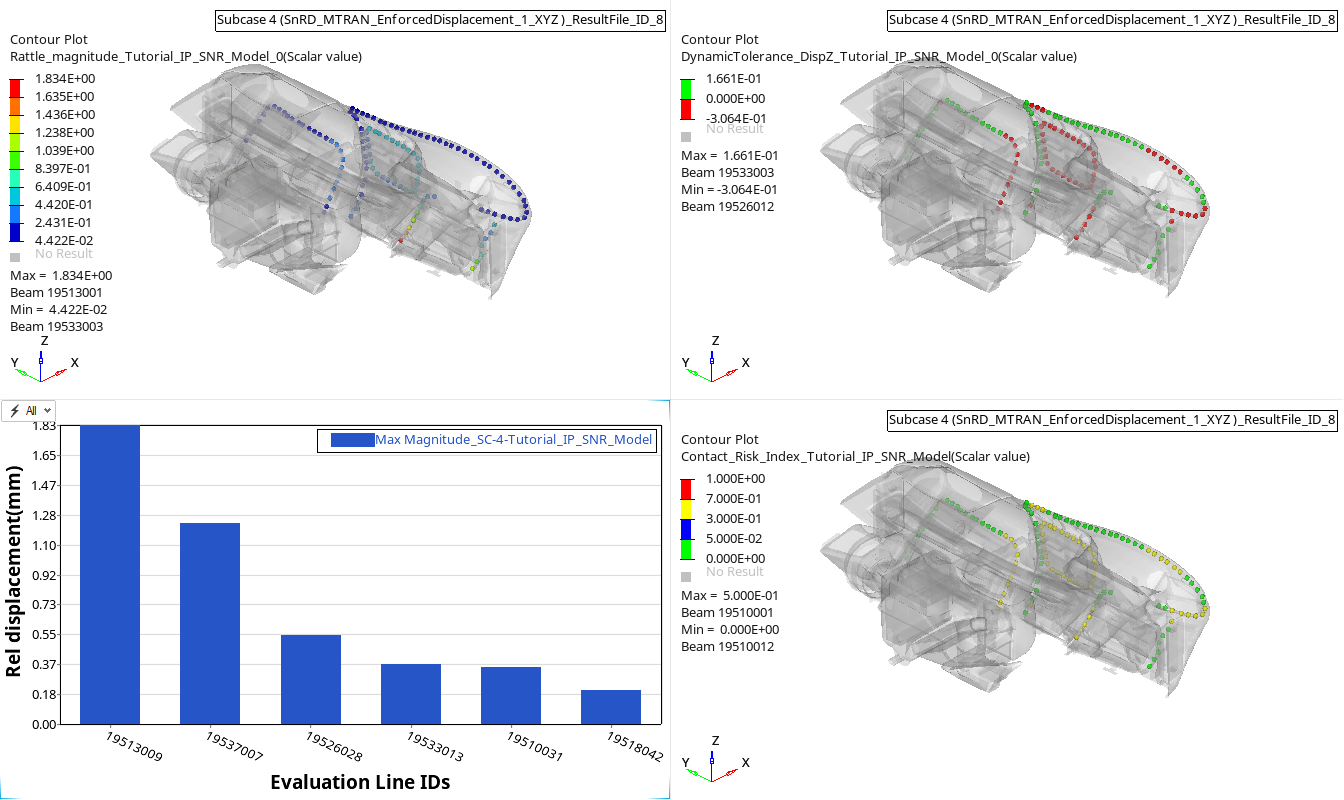 Figure 10. Rattle Summary Dynamic
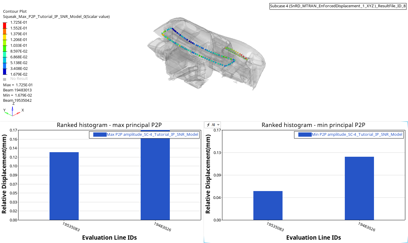 Figure 11. Squeak Summary Dynamic
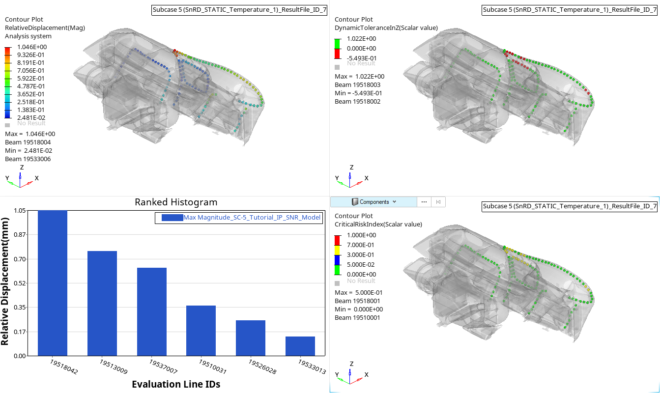 Figure 12. Rattle Summary Thermal
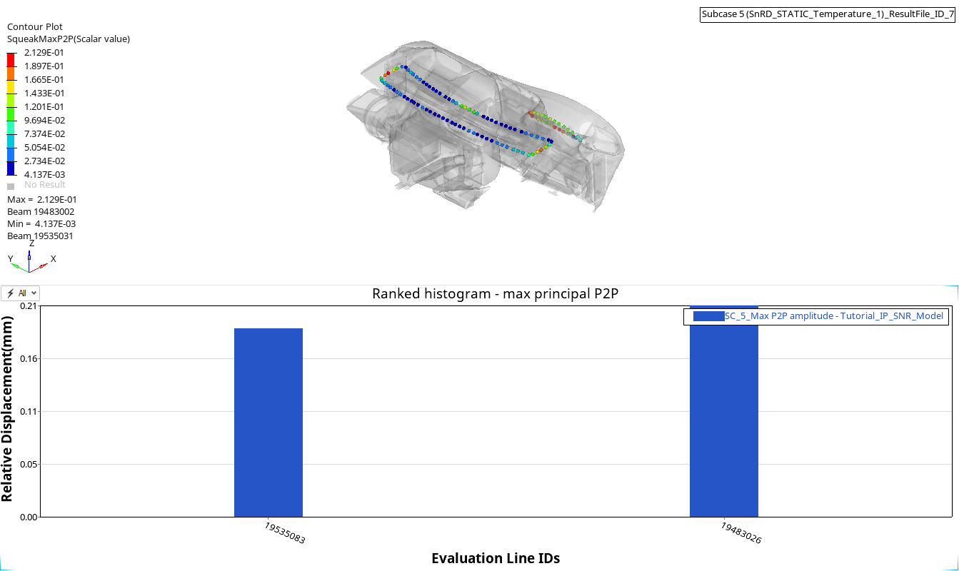 Figure 13. Squeak Summary Thermal
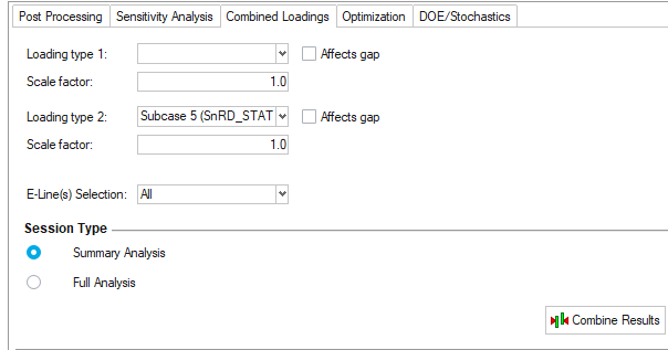 Figure 14.
 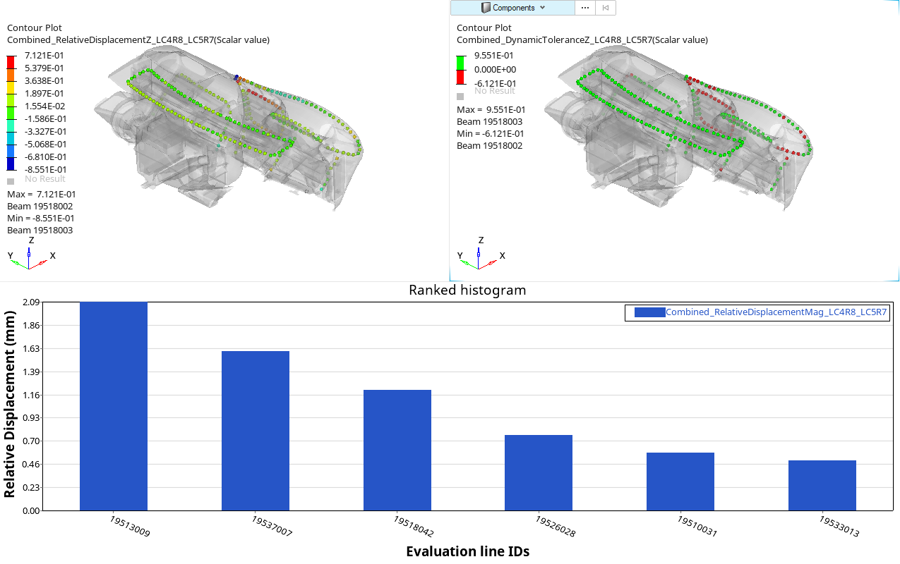 Figure 15.
 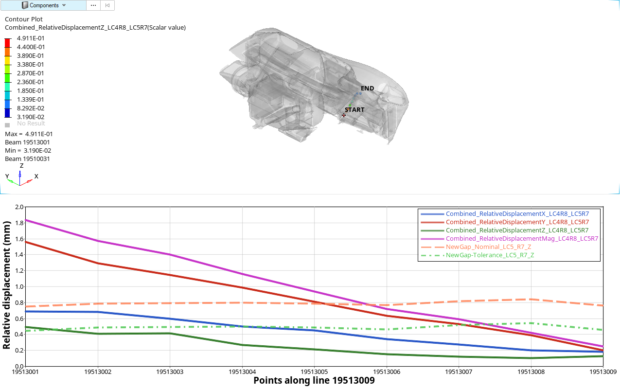 Figure 16.