Use SnRD to identify, evaluate, and eliminate squeak and rattle issues.
During the first S&R screening risk analysis, several input data were lacking for
the different interfaces. At that time, no gap or material properties were defined
yet. Now the design team has more information for each of the E-lines that have been
analysed:
Rattle Lines:
The gap and tolerances are now defined from the styling and
Engineering departments.
These dimensions can now be imported into SnRD and used for updating
the existing model.
Squeak Lines:
Material choices are more mature, therefore the stick slip testing
data can be search for and applied for relevant E-lines.
The stick slip data available in different sources (Ziegler data
base, own data base etc.) can be imported into SnRD for update of
existing model.
The objectives of this tutorial are:
Create FE model prepared for analyzing.
Create E-Lines using Auto & Manual
methods-
6 Rattle lines
2 Squeak lines
A dynamic loadcase, with user defined multi direction loading data.
Run analysis, post process and perform sensitivity study.
Before you begin, copy the file(s) used in this tutorial to your working
directory:
The selected model, DTS, and material file are imported to the
session.Figure 2.
Import Geometric Lines File
In this step, you will import the geometric lines file.
From Setup group, select Define Interface > Import Geometry File.
Figure 3.
A file browser dialog opens.
Browse and select the GeometricLines.stp file.
The geometry lines file is imported into the session.Figure 4.
Create E-Lines
In this step, you will use the Create E-Lines tool to create
E-Lines at the interfaces.
Below are the E-Lines you will create
in this step.
Table 1.
Method
Line Type
Gap Direction
Main Component
Secondary Component
Interface Name
Manual
Rattle
In plane to Main
IP Substrate
Glove Box
GloveBox_To_IPsubstrate
Manual
Squeak
In plane to Main
IP Substrate
Dashboard Panel
Ipsubstrate_To_Dashboardpanel
Manual
Rattle
In plane to Main
IP Substrate
Control Panel Upper
IPsubstrate_To_ControlpanelUpper
Manual
Rattle
Normal to Main
Radio Panel
Lower Control Panel
Radiopanel_To_ControlPanelLower
Manual
Rattle
In plane to Main
Driver Side Panel
Lower Control Panel
DriverSidepanel_To_Controlpanellower
Manual
Rattle
In plane to Main
Driver Side Panel
IP Substrate
DriverSidepanel_To_IPsubstrate
Manual
Rattle
In plane to Main
Lower Control Panel
IP Substrate
IPsubstrate_To_Controlpanellower
Manual
Squeak
Normal to Main
Speedometer
Control Panel Upper
Speedometer_To_ControlPanelUpper
Create E-Lines manually.
From the Setup group, select the
Create E-Line tool.
Figure 5.
A guide bar opens.
Deactivate to manually
create E-Lines.
For Main Components, select IP Substrate.
For Secondary, select Glove Box.
Tip: Press Tab to toggle between
selections.
For Lines, select the geometric line present at the edge of the Glove
Box component.
Click .
E-Lines are created at the interface and will
be highlighted in yellow.Figure 6.
Repeat the substeps above to create a Squeak line between the IP
Substrate and Dashboard Panel.
Once all E-Lines are created, your model
should look like Figure 7.Figure 7.
Realize E-Lines
In this step, you will use the Manage E-Lines tool to realize all
E-Lines.
From the Setup group, select Manage E-Lines > Review E-Lines tool.
Figure 8.
The Review E-Line table opens.
Map the correct interface from the DTS file to the created E-Lines and ensure all other options, like Gap direction, are
correct.
Figure 9.
Optional: If an E-Line status is yellow, click to realize and update E-Lines.
Go to the Material Mapping tab and select the following materials for the two
squeak E-Lines.
IPSubstrate_To_Dashboardpanel
For Main Material, select PPTD_20.
For Secondary Material, select
PPTD_20.
Speedometer_To_ControlPanelUpper
For Main Material, select PPTD_20.
For Secondary Material, select ABS.
Define Dynamic Loadcase
In this step, you will create a Dynamic loadcase.
From Setup group, select Dynamic
Event.
Figure 10.
From the graphics area, select the node shown in Figure 11.
Figure 11.
A microdialog opens.Figure 12.
Verify Displacement (D) is selected as load type.
For Load Curve, select From File.
For load directions, select X, Y,
and Z.
Click .
A file browser dialog opens.
Browse and select the Excitation_XYZ.csv file from the
003_loads folder.
The required load collectors and other entities required for the
simulation are created. The newly created loads are displayed in the
Curve Editor dialog.
In the Curve Editor dialog, review the load curves and
close the dialog.
Figure 13. Figure 14.
Tip: You can use the Model Browser to view
the new entities.
Review Loadcase and Export Solver Deck
Review the Dynamic Loadcase.
From the Analyze group, select Review All
Loadcase.
Figure 15.
The Load Step Table dialog opens.Figure 16.
Verify the Export checkbox is enabled for the
SnRD_Dyn_Disp_#_XYZ entry.
Click Close.
From the Analyze group, select Export
OptiStruct Solver File.
Figure 17.
The Model Export dialog opens.Figure 18.
Click Export.
A folder selection dialog opens.
Browse and select the required folder.
The OptiStruct solver deck is exported to
the selected folder.
Click Close to close the Model
Export dialog.
Use the exported .FEM solver deck to
solve in the OptiStruct solver. Once completed, two output
files are generated: .H3D and .PCH. These
files will be used in the Post Processing of results.
Import Model and Results File
In this step, you will use the SnRD Post to post process the
results.
Open HyperView.
From the menu bar, click File > Load > Preferences File.
The Preferences dialog opens.
In the Preferences dialog, select Squeak &
Rattle and click Load.
The SnRD menu is opened in the HyperView client.
Select SnRD > SnRD-Post.
The SnRD Post Processing tool opens.Figure 19.
Using the file browse option , select the OptiStruct
solver file which was exported in Export OptiStruct Solver File for Model File.
Note: Pre output CSV file containing the E-Lines definition is sourced automatically.
Click .
A file browser dialog opens.
Select the tutorial_ip_snr_model.pch file from the
tutorials folder.
A working status dialog opens while reading the PCH data.Figure 20.
Enable the checkbox for the subcase in the Subcase selection table.
Click in the Save Session File entry field.
Browse and select the required folder where the post processing session and
data will be stored.
Once complete, your entries in the table should match Figure 21.Figure 21.
Post Process Results
In this step, you will perform a Full Analysis to understand the squeak and rattle risks in the model.
In the Post Processing tab, define the following parameters.
For Analysis Type, select Rattle &
Squeak.
For Line(s) to Evaluate, select All.
For % statistical evaluation, enter 0.
For Session Type, select Full Analysis.
Click Execute.
Note: Execution of Full Analysis will take a considerable
amount of time to chart histograms and plot contours based on the machine's
performance.
An execution success message opens.Figure 22.
Click Close.
Full analysis creates 11 pages containing all the details. The summary for Rattle
analysis can be found on Page one.Figure 23. Rattle Summary Dynamic
Summary for Squeak analysis can be found on Page nine.Figure 24. Squeak Summary Dynamic
Evaluate Results
In this step, you will study the histograms and contour plots to understand results
and complete squeak and rattle risk evaluation.
From page one of the Rattle Summary Dynamic, you can see the
Rattle line ID 19513009 has the maximum relative displacement. You will perform
Sensitivity Analysis to evaluate the effects of modes on the relative
displacements.
Navigate to page five to view the Rattle Detailed Dynamic - Line ID 19513009
details.
Figure 25.
The Relative Displacement of 1.85915 mm at the point 19513001. This is higher
than the Gap and (Gap - Tolerance) values. This indicates a risk of rattle at
this particular interface of Driver Side Panel - Lower Control Panel.
Click the Sensitivity Analysis tab.
Define the following parameters.
For Result File, select
Tutorial_IP_SNR_Model.pch.
For Subcase Name, select Subcase 4
(SnRD_MTRAN_EnforcedDisplacement_1_XYZ).
For Modal Result File (.H3D), select
Tutorial_IP_SNR_Model.h3d.
In the E-Line Selection section, define the following parameters.
For E-Lines, select
19513009.
For Select Pair, select Line check box.
For Select Direction, select Z.
Click Load Time History.
A working window opens stating the process of plotting relative
displacement.Figure 26.
Once complete, the relative displacement plots for all the points in the
line are plotted.Figure 27.
Under the Modal Contribution panel, click Analyze.
A working dialog opens stating the process of plotting Relative Modal
Contribution.Figure 28.
Relative Modal Contribution - Line 19513009 - z is created with modes,
contour and relative displacement plots for the line.Figure 29.
From the Modes plot, the Mode-4 of value 26.5 Hz is the highest
contributing factor for the rattle issue.
Click Modal Sensitivity under the Modal Sensitivity
Studies panel.
Figure 30.
Select Exclude from the Select Contributor(s) to
list.
Enter 50 for % to Exclude value.
Enable the checkbox for mode 4 under the Mode # column.
Click Analyze.
The Modal Sensitivity for Line (MSL) - Line ID 19513009 -z page is
created in the session with the Max Relative Displacement (mm) values plotted
against all the interface points.Figure 31.
The relative displacement is reduced when the mode 4 is excluded by
50%.
Repeat the above steps to study the remaining lines in the model.
 to open additional
options.
to open additional
options.
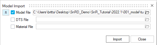 Figure 1.
 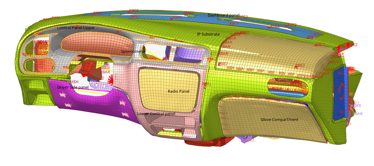 Figure 2.
  Figure 3. A file browser dialog opens.
 Figure 4.
  Figure 5. A guide bar opens.
 to manually
create E-Lines.
to manually
create E-Lines.
 .
E-Lines are created at the interface and will be highlighted in yellow.
.
E-Lines are created at the interface and will be highlighted in yellow. Figure 6.
  Figure 7.
  Figure 8. The Review E-Line table opens.
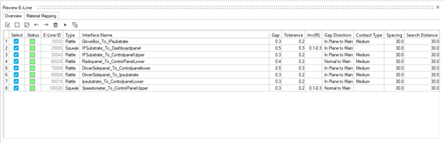
 Figure 10.
 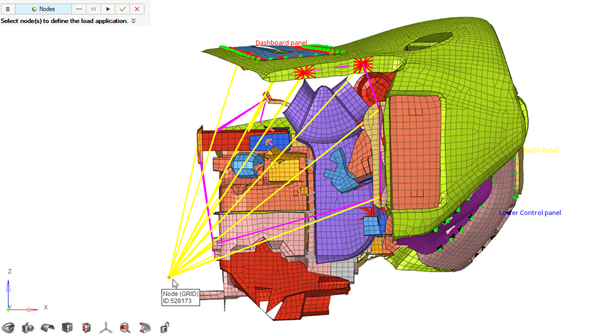 Figure 11. A microdialog opens.
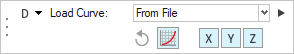 Figure 12.
 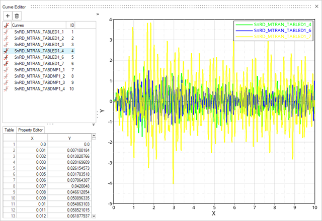 Figure 13.
 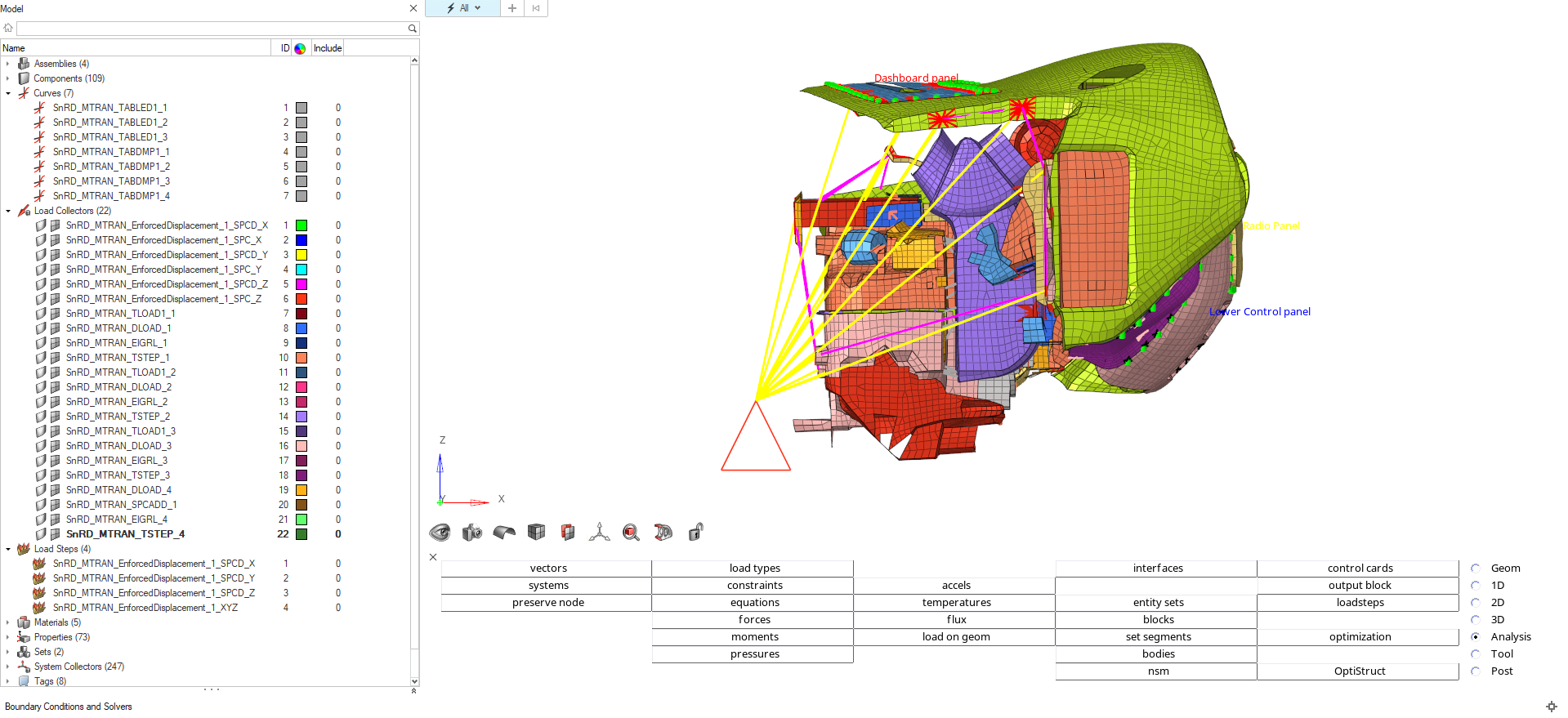 Figure 14. Tip: You can use the Model Browser to view the new entities.
 Figure 15. The Load Step Table dialog opens.
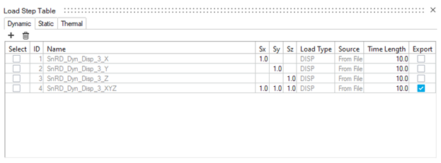 Figure 16.
  Figure 17. The Model Export dialog opens.
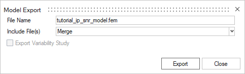 Figure 18.
 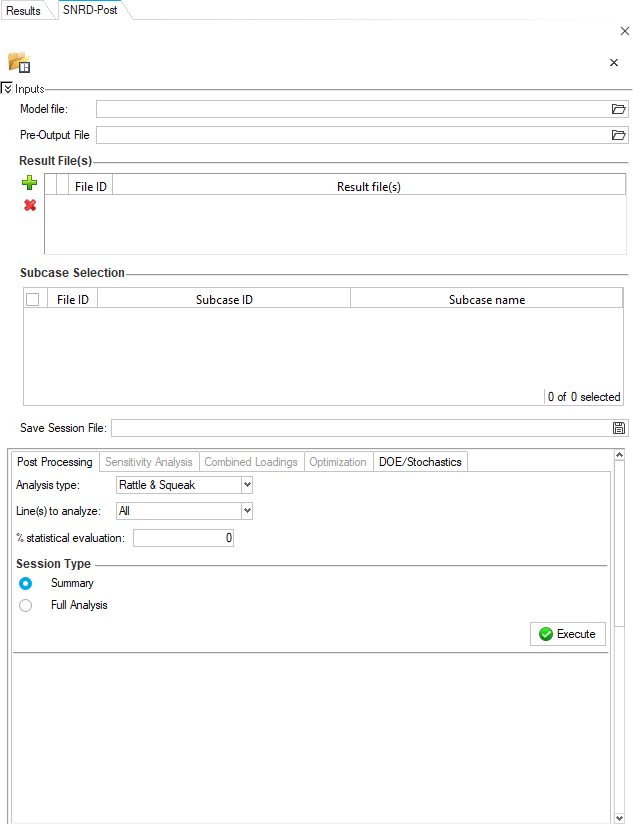 Figure 19.
  , select the OptiStruct
solver file which was exported in Export OptiStruct Solver File for Model File.
Note: Pre output CSV file containing the E-Lines definition is sourced automatically.
, select the OptiStruct
solver file which was exported in Export OptiStruct Solver File for Model File.
Note: Pre output CSV file containing the E-Lines definition is sourced automatically. .
A file browser dialog opens.
.
A file browser dialog opens.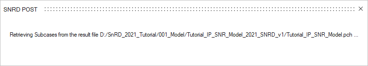 Figure 20.
  in the Save Session File entry field.
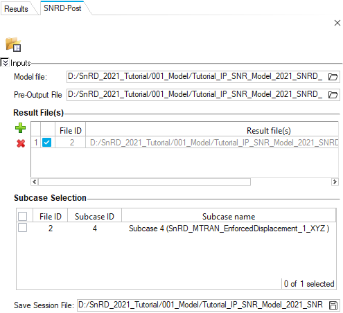 Figure 21.
 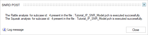 Figure 22.
 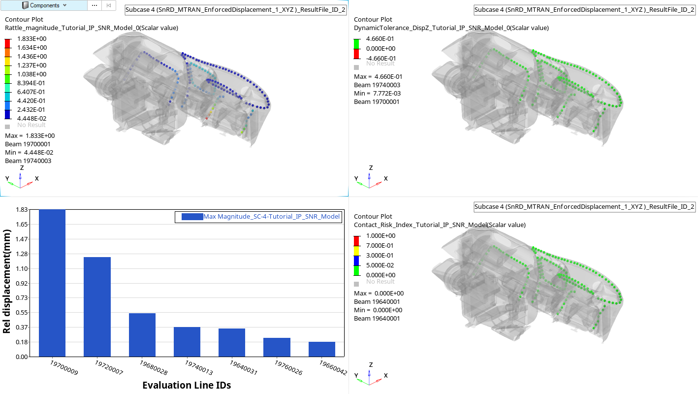 Figure 23. Rattle Summary Dynamic
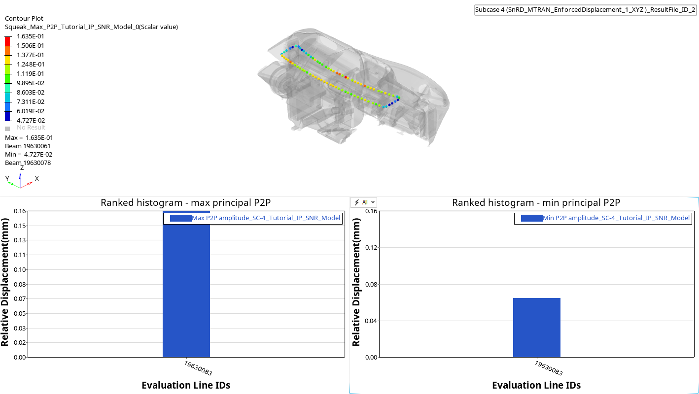 Figure 24. Squeak Summary Dynamic
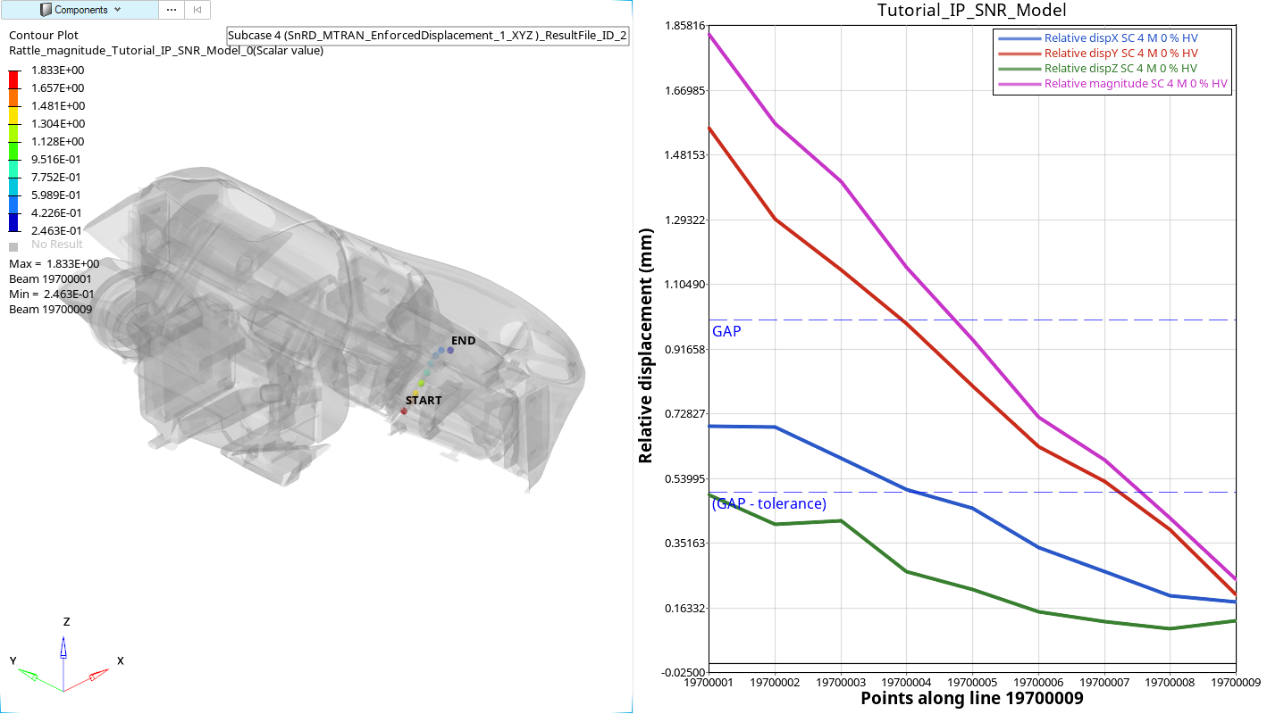 Figure 25. The Relative Displacement of 1.85915 mm at the point 19513001. This is higher than the Gap and (Gap - Tolerance) values. This indicates a risk of rattle at this particular interface of Driver Side Panel - Lower Control Panel.
 Figure 26.
 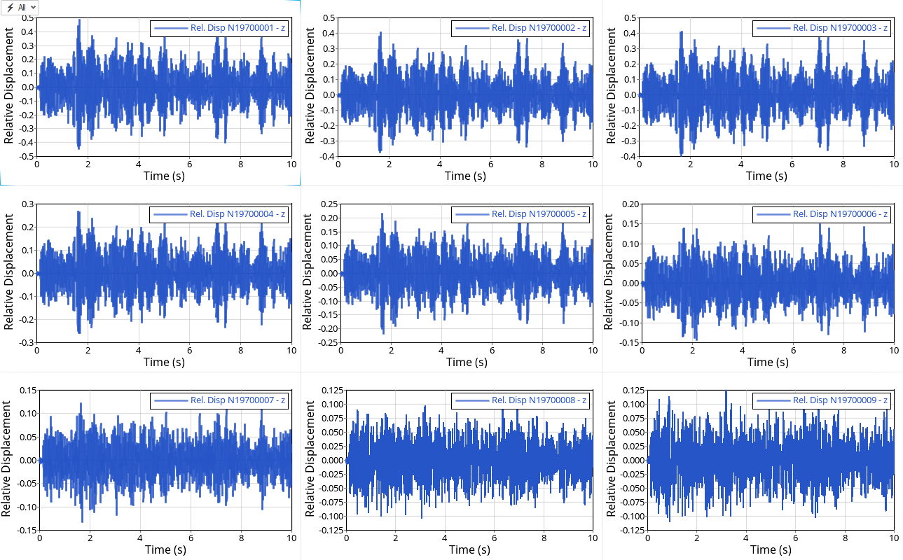 Figure 27.
  Figure 28.
 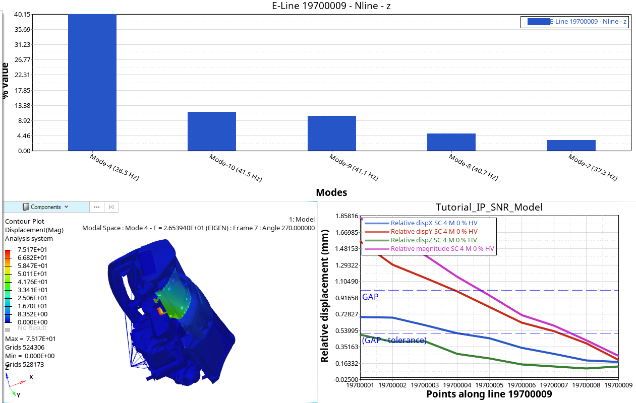 Figure 29.
 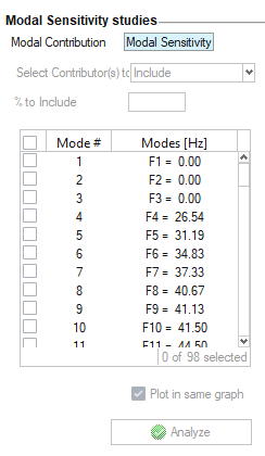 Figure 30.
 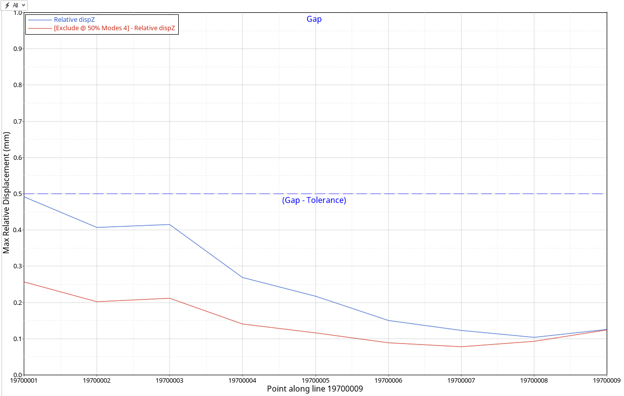 Figure 31.