Feko is a comprehensive electromagnetic solver with multiple solution methods that is used for electromagnetic field analyses
involving 3D objects of arbitrary shapes.
3D views are used to display and interact with the model. You can zoom, rotate and pan around a 3D model using the keyboard,
mouse or a combination of both. You can use a 3D mouse, specify a view or select specific parts of a model. Multiple 3D
views are supported.
Define field or current data using either far field data, near field data, spherical mode data or PCB current data. Use
the field/current definition when defining an equivalent source or a receiving antenna.
Define a medium with specific material properties, import a predefined medium from the media library or add a medium from
your model to the media library.
Defined media can be applied to the model in various ways. Some media settings are applied to regions, others on faces
and wires. The rules for defining media varies between the different solution methods.
Use a periodic boundary condition (PBC) to analyse infinite periodic structures. A typical application of PBC is to
analyse frequency selective surface (FSS) structures.
Create an arbitrary finite antenna array that consists of an array of contributing elements, either with direct feeds for
each element or via indirect coupling, and solve with the efficient domain Green's function method (DGFM).
Use the windscreen tools to define a curved reference surface constrained by a cloud of points, normals and optional U′V′ parameters. The constrained surface is then used as a reference to create a work surface where windscreen layers and curved
parameterised windscreen antenna elements can be created.
Many electromagnetic compatibility and interference problems involve cables that either radiate, are irradiated or cause
coupling into other cables, devices or antennas. Use the cable modelling tool and solver to analyse the coupling and radiation.
For a frequency domain result, the electromagnetic fields and currents are calculated at a single frequency or frequency
range. When the finite difference time domain (FDTD) solver is used, the frequency must be specified to convert the native time domain results to the frequency domain.
The excitation of an antenna is normally specified as a complex voltage, but it may be useful to specify the total radiated
or source power instead. The result is then scaled to yield the desired source power level.
A port is a mathematical representation of where energy can enter (source) or leave a model (sink). Use a port
to add sources and discrete loads to a model.
Perform multiple solutions for a single model using multiple configurations. Multiple configurations remove the requirement
to create multiple models with different solution requests.
A characteristic mode configuration results in a characteristic mode analysis (CMA) request. The analysis is based
on the numerical calculation of a weighted set of orthogonal mode currents.
Use an infinite plane or half-space to model a ground plane efficiently. The number of triangles in the model is reduced
as the ground plane is not discretised into triangles.
Domain connectivity approach allows meshes of specific parts to be treated as if “connected” during MoM and MoM/MLFMM solutions in places where the borders of the meshes are close together, even if the mesh vertices on those borders
are not coincident.
A CADFEKO.cfm file can be imported into EDITFEKO to make use of more advanced features available in EDITFEKO and to directly edit the .pre file for more flexible solution configurations.
During the design process, the development of a model can introduce a range of issues that can lead to a non-simulation-ready
model. Use the validation toolset to verify that the model is simulation-ready or to search, detect and flag discrepancies.
The default solver used in Feko is the method of moments (MoM) - surface equivalence principle (SEP). A solver is specified per model, per face or per region, and depends on the solver in question.
CADFEKO has a collection of tools that allows you to quickly validate the model, for example, perform calculations using
a calculator, measure distances, measure angles and export images.
EDITFEKO is used to construct advanced models (both the geometry and solution requirements) using a high-level scripting language
which includes loops and conditional statements.
One of the key features in Feko is that it includes a broad set of unique and hybridised solution methods. Effective use of Feko features requires an understanding of the available methods.
Feko offers state-of-the-art optimisation engines based on generic algorithm (GA) and other methods, which can be used
to automatically optimise the design and determine the optimum solution.
Feko writes all the results to an ASCII output file .out as well as a binary output file .bof for usage by POSTFEKO. Use the .out file to obtain additional information about the solution.
CADFEKO and POSTFEKO have a powerful, fast, lightweight scripting language integrated into the application allowing you to create
models, get hold of simulation results and model configuration information as well as manipulation of data and automate
repetitive tasks.
Perform multiple solutions for a single model using multiple configurations. Multiple configurations remove the requirement
to create multiple models with different solution requests.
Define an S-parameter configuration and add it to the model.
Add an S-parameter configuration using one of the following workflows:
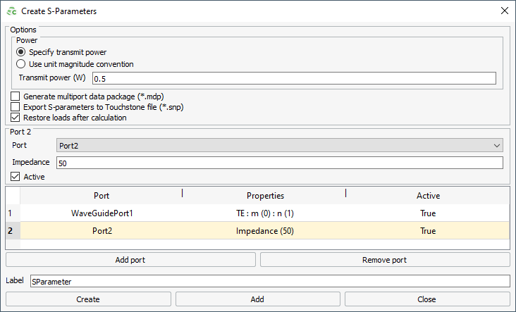
On the Request tab, in the
Configurations group, click the S-parameter Configuration icon.
In the configuration list, click the icon. Select S-parameter Configuration from the
menu .
In the Power group select one of the following:
Select Specify transmit power to specify the
transmit power for all the ports when calculating the requests associated
with the S-parameter request.
Select Use unit magnitude convention to use the
unit magnitude convention to calculate the requests associated with the
S-parameter request.
Note: The S-parameter matrix
result is not affected when selecting the power option, only the fields
or current requests associated with the S-parameter request is altered
based on the power information.
[Optional] In the Options group, select the
Export S-parameters to Touchstone file check box to
export the S-parameters to a .snp file.
For each S-parameter configuration, a separate Touchstone file is created.
The file name is in the form
<FEKO_base_filename>_<requestname>(k).snp where:
FEKO_base_filename
file name of the model
requestname
request name
n
number of ports
k
a counter (integer) to distinguish between the results of
multiple requests with the same name and the same number of
ports.
Note:
Feko does not normalise the S-parameter
values to a global reference impedance when exporting the S-parameters
to a Touchstone file. The values are referenced to the impedance
specified on each port.
CAUTION:
Some industry tools that use the Touchstone format often
assume that all values are referenced to a common impedance. When exporting
S-parameters for use in an industry tool that supports only a single
reference impedance, specify the reference impedance for each port to ensure
the correct interpretation.
[Optional] In the Options group, select the
Restore loads after calculation check box to remove
the loads once the S-parameter calculation is complete.
In the Port column, from the
drop-down list, select the port.
In the Properties column, specify
the following:
For waveguide ports, specify the type (TE1 / TM2/ TEM3), indices and rotation of the
mode.
For ports other than waveguide and FEM modal ports, specify the reference impedance. If no impedance is
specified, a default reference impedance of 50 Ohm is used.
In the Active column, select the check box to use the
port as a “source” (else the port is only a “receiving” or “sink”
port).
Note: For example, if a Port1 and Port2 is
defined, but only Port1 is active, only S11
and S21 are calculated.
During the calculation of S-parameters, the specified reference impedances
are added as loads to the ports. These loads remain in place after the S-parameter
calculation. If the loads are removed once the S-parameter calculation is complete
and there are subsequent output requests, such as near fields, the full matrix
computation and LU decomposition steps will be repeated for the MoM solution method. This is typically the most
time-consuming step in the analysis. It must be noted that should near fields be
requested, and the loads remain, the near fields will be lower in magnitude due to
the losses in the loads.
In the Label field, add a unique label for the
request.
Click Create to request the S-parameter results
and to close the dialog.
The port numbers in an S-parameter solution are indexed
based on the order of appearance in the port list on the Create
S-parameters dialog, and not according to the label of the selected
port.