SS-V: 9002 Wave Propagation in Loaded Waveguide

Test No. VE03Propagation of the fundamental mode wave in a loaded waveguide

Definition

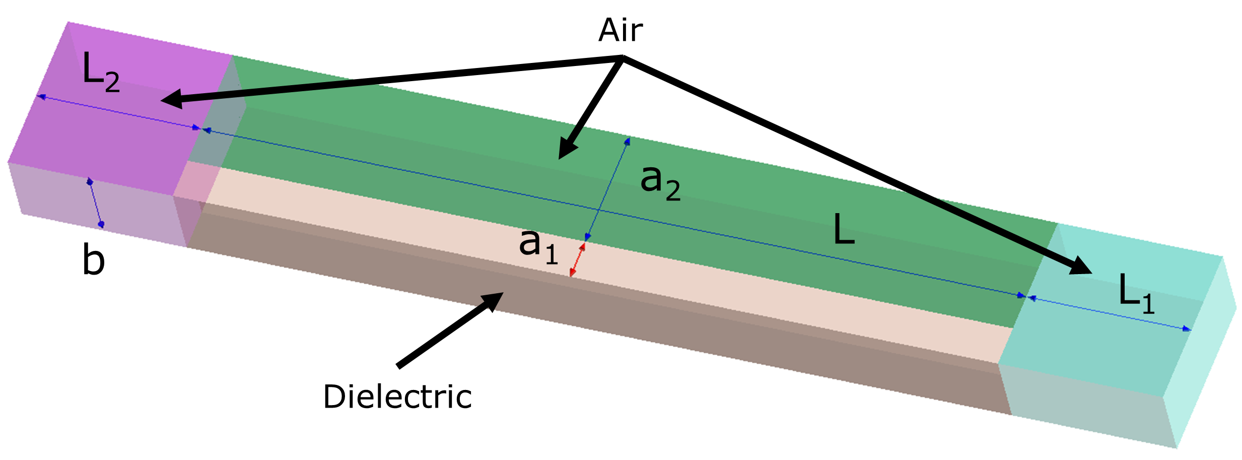
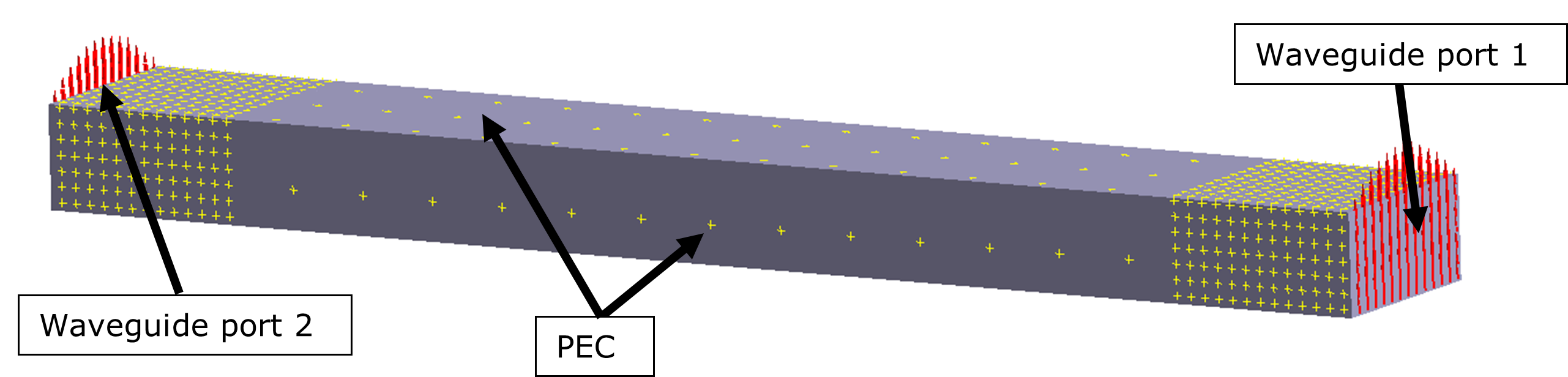
The details of the model are:

Figure 1: a1 = 5mm, a2 = 15mm, a = a1 + a2, b = 10 mm, L = 100 mm, L1 = L2 = 20 mm
All side walls are at the PEC (Perfect Electric Conductor) conditions, and end faces are waveguide ports

The material properties are:

Properties: Value
Dielectric relative permittivity ( $ε_{r}$ ): 4.0
Dielectric relative permeability ( $μ_{r}$ ): 1.0
Air relative permeability ( $ε_{r}$ ): 1.0
Air relative permeability ( $μ_{r}$ ): 1.0

Reference Solution

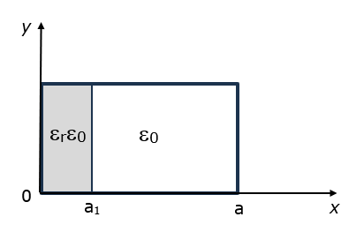
Figure 3. Cross section of the waveguide

In both the dielectric and the air, the wave is propagating with the same wave number and common factor is

e x p (- j β z)

, where

β

is the longitudinal wave number. We are looking for the TE_m0 modes (the one with m = 1 is the fundamental mode), which means that there is no dependence on y^¹.

Equations for longitudinal magnetic field become:

(\frac{\partial^{2}}{\partial x^{2}} + {k_{D}}^{2}) H_{z} = 0 for 0 \leq x \leq a_{1}

(\frac{\partial^{2}}{\partial x^{2}} + {k_{A}}^{2}) H_{z} = 0 for a_{1} \leq x \leq a

Where,

{k_{A}}^{2} = {k_{0}}^{2} - β^{2}

and

{k_{D}}^{2} = {ε_{r} k_{0}}^{2} - β^{2}

Depending on the combination of the model parameters both ${k_{A}}^{2}$ and ${k_{D}}^{2}$ are positive or ${k_{D}}^{2}$ is positive and ${k_{A}}^{2}$ is negative.

In the first case the value of $β$ is obtained from the solution of the following equation:

k_{A} \tan (k_{D} a_{1}) + k_{D} \tan (k_{A} a_{2}) = 0

This is after substituting ${k_{A}}^{2}$ and ${k_{D}}^{2}$ from their definitions^¹.

In the case of the negative value of ${k_{A}}^{2}$ in a similar way the value of $β$ is obtained from the solution of the equation (this case is complementary to the one in Pozar^¹):

k_{A} \tan (k_{D} a_{1}) + k_{D} \tan h (k_{A} a_{2}) = 0

Where,

{k_{A}}^{2} = - {k_{A}}^{2} = - {k_{0}}^{2} + β^{2}

and it is positive.

In the first case the electric field distribution is:

In the second case the electric field distribution is:

Results

In the case of

f = 7.5 GHz {k_{A}}^{2} > 0

and equation (1) is in effect, while at the

f = 10 GHz {k_{A}}^{2} < 0

and equation (2) should be used.

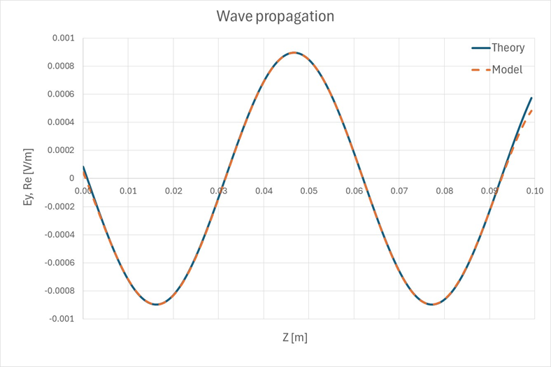
Figure 6. Electric field $E_{y} (Z) (R e)$ distribution at f = 7.5GHz with Waveguide Port 1 active

Figure 7. Comparison of theoretical and modeled electric field distribution along the line in above figure

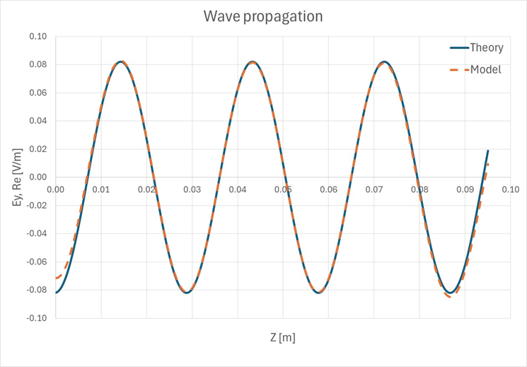
Figure 8. Electric field $E_{y} (Z) (R e)$ distribution at f = 10GHz with Waveguide Port 1 active

Figure 9. Comparison of theoretical and modeled electric field distribution along the line in above figure

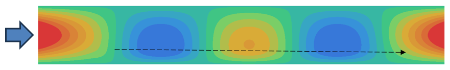
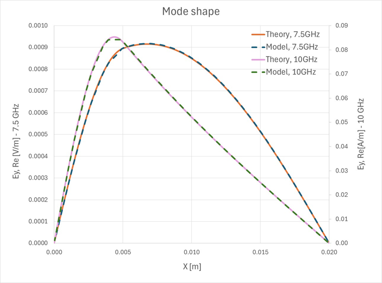
The above formulas for the field distribution are illustrated in the following graph (x is orthogonal to the direction of the wave propagation here and the sampling line goes through the maximum of the field distribution):

Figure 10. Comparison of theoretical and modeled electric field distribution for fundamental mode at different frequencies

¹ Pozar, D.M., Microwave Engineering, 4th Edition, John Wiley & Sons, Inc., 2012, p.119.