Test No. VE04Analysis of modes in resonator with two
materials
Definition
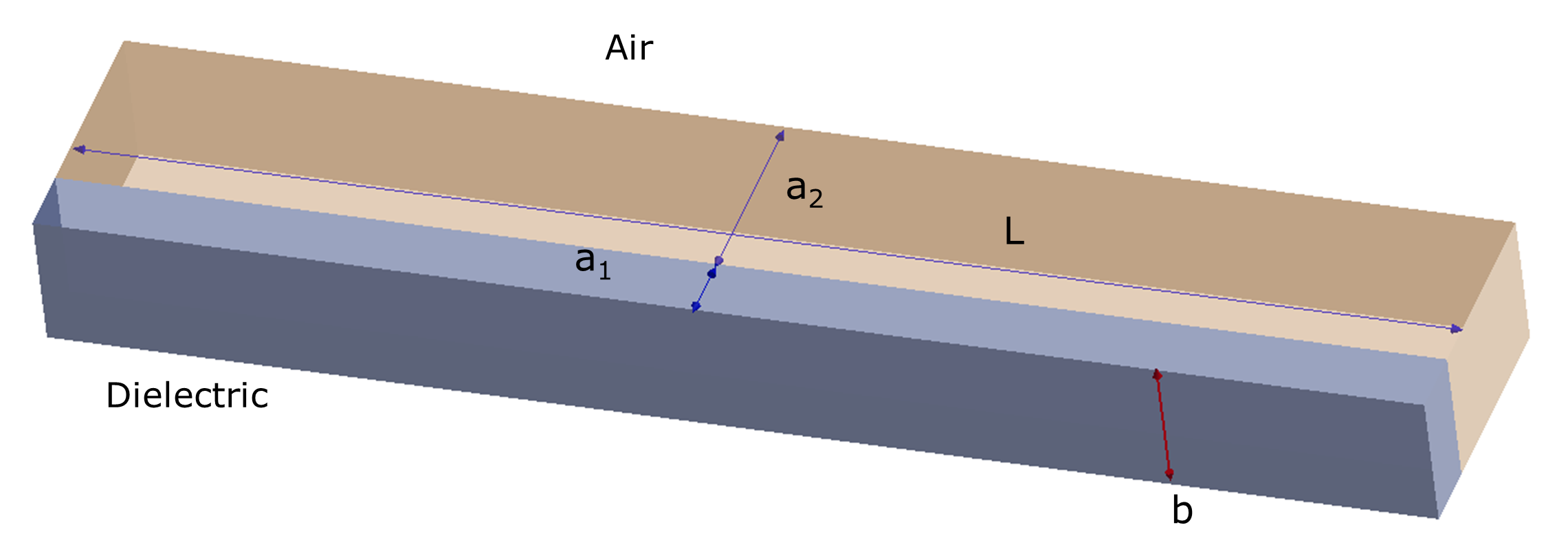
Figure 1. The details of the model are:
Figure 1: a1 = 5mm, a2 = 15mm, a = a1 + a2, b = 10 mm, L =
100 mm
All walls are under PEC (Perfect Electric Conductor) conditions
The material properties are:
Properties
Value
Dielectric relative permittivity ()
4.0
Dielectric relative permeability ()
1.0
Air relative permeability ()
1.0
Air relative permeability ()
1.0
Reference Solution
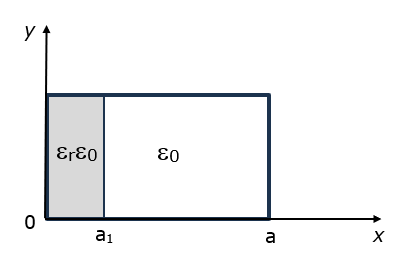
Figure 2. Cross section of the resonator We are looking for the modes (the one with l=1 is the fundamental
mode), which means that there is no dependence on y1.
Equations for longitudinal magnetic field become:
Where,
and
Depending on the combination of the model parameters both and are positive or is positive and is negative.
In the first case the value of is obtained from the solution of the following
equation:
This is after substituting and from their definitions above1.
In the case of the negative value of in a similar way the value of is obtained from the solution of the equation (this
case is complementary to the one in Pozar1):
Where,
and it is positive.
The roots of those transcendental equations can be found numerically or graphically
depending on required accuracy.
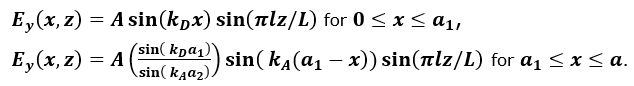
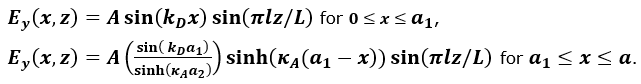
In the first case the electric field distribution is:Figure 3. In the second case the electric field distribution is:Figure 4.
Results
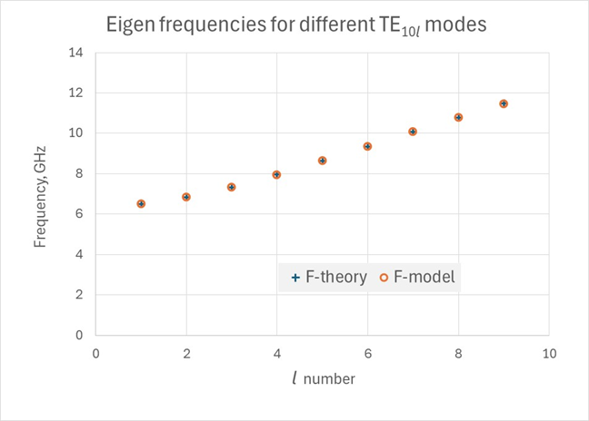
Comparison of the theoretical resonant frequencies for the modes with those obtained in the modeling is
presented in the picture below.Figure 5. Comparison of theoretical and model resonant frequencies
The z dependence of the field is simple and was followed in the
solution with high accuracy. It is interesting to check, how accurate is the
x dependence reproduced in the model. Electric field magnitude was output
at fixed z corresponding to one of its maximums and normalized to that
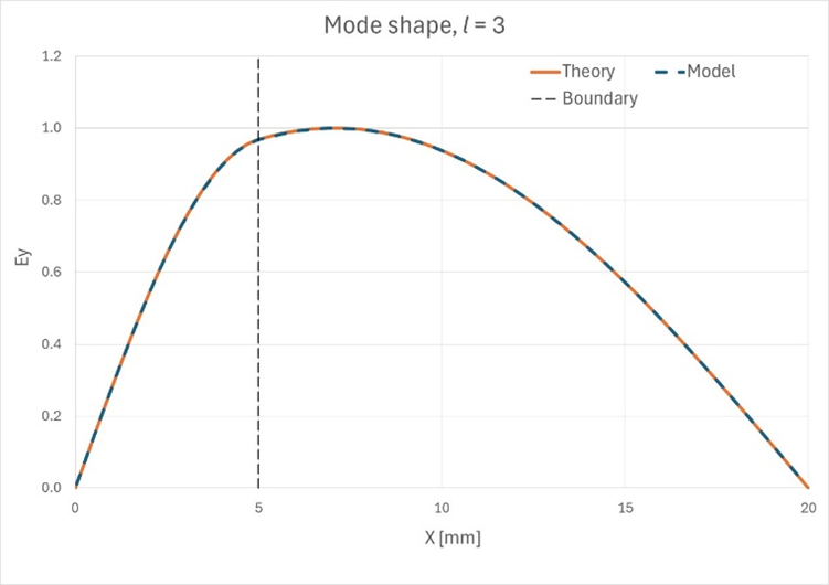
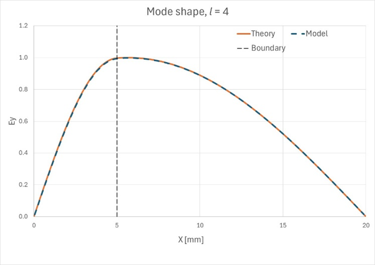
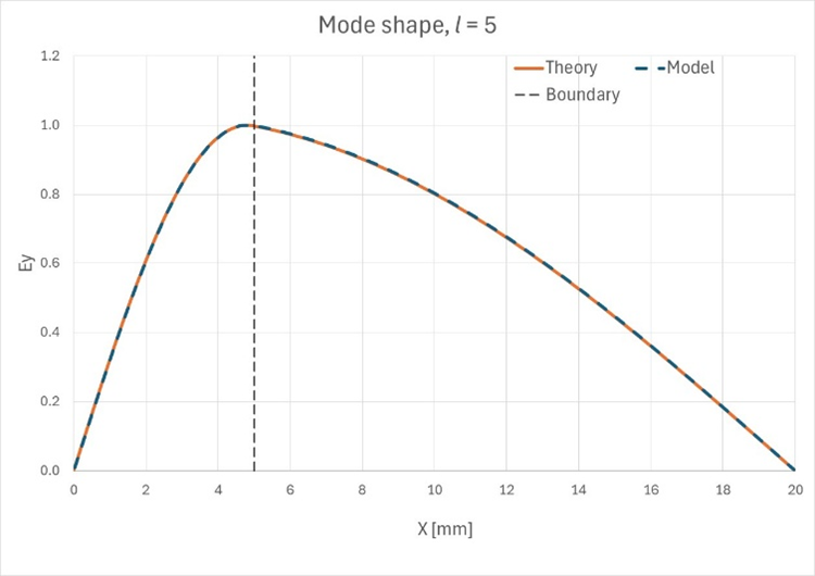
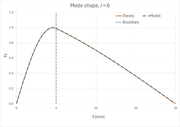
maximum. Below, this is illustrated for the case of l=3.Figure 6. Electric field magnitude distribution for the mode
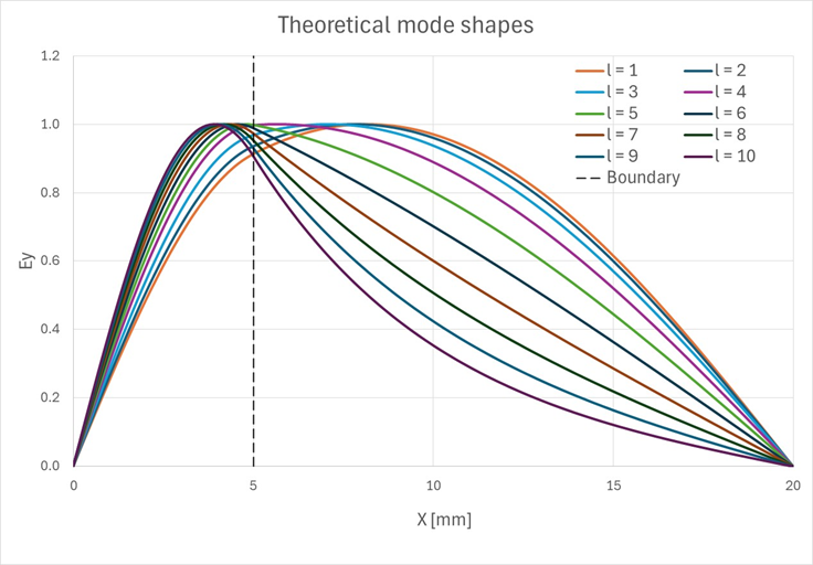
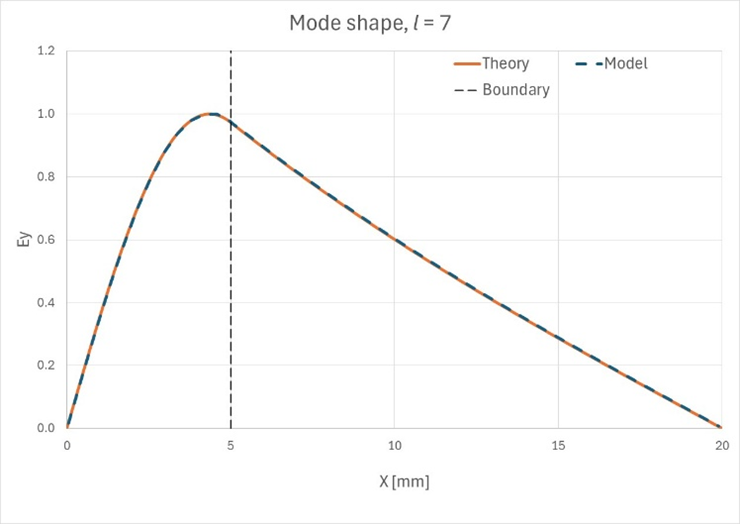
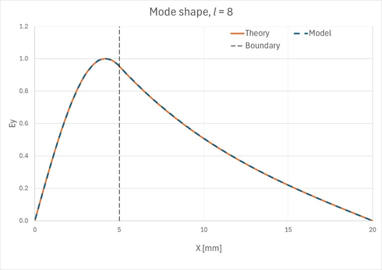
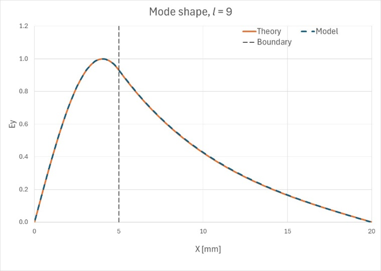
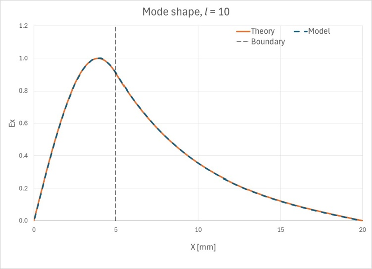
As it is described above for some values of l the solution on both
sides of the boundary is described by the sin function, for other values (in our
case – starting from l=7) the sin function in the area with air switches to
the hyperbolic sin. This can be observed in the figure below.Figure 7. Mode shapes for the first 10 modes.
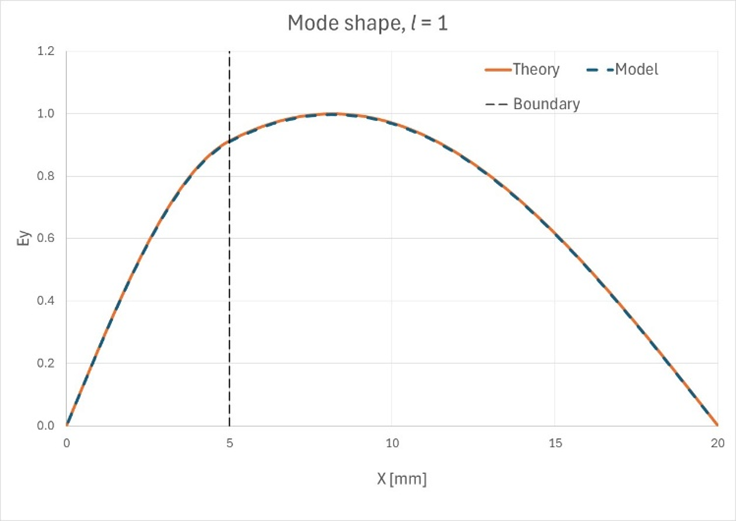
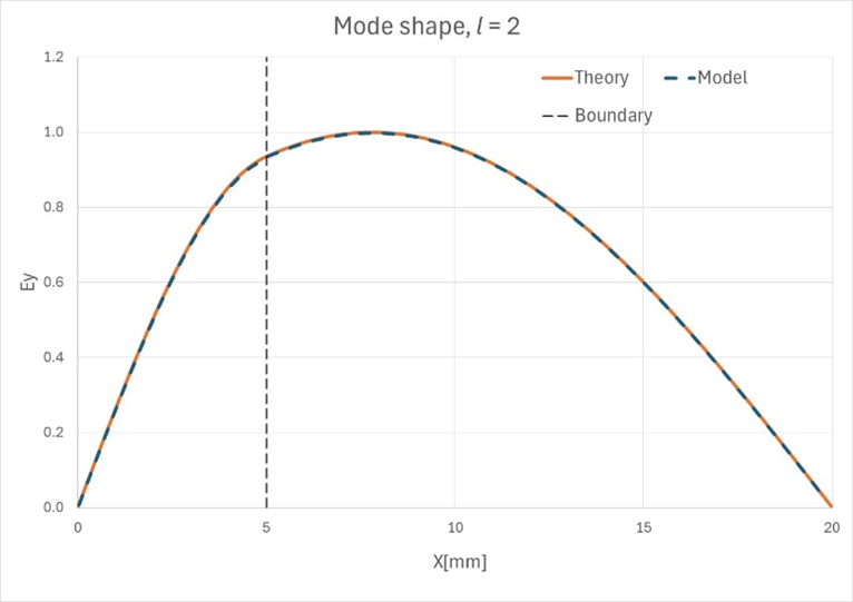
Figure 8. Match between theoretical and observed mode shapes for the first 10 modes
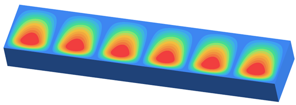
First 6 modes are of the type. Field distribution for the mode is shown below.Figure 9. Electric field magnitude for the mode
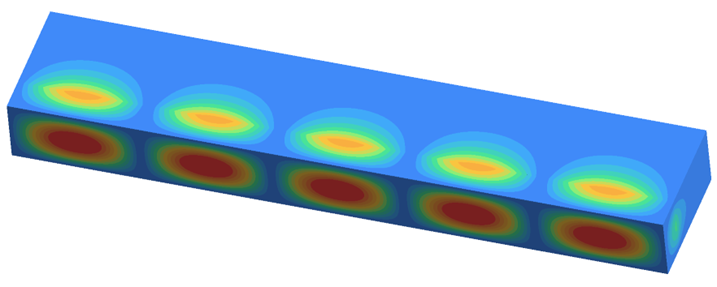
The higher modes with the electric field that is not uniform in y
direction are a mixture of the TE and TM waves.Figure 10. Electric field magnitude for the mode number 12
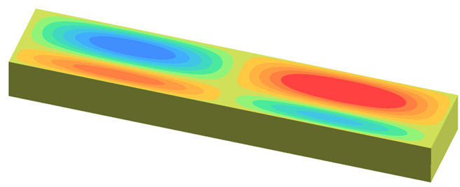
If the field is uniform in y direction, the modes still can be
classified in terms of TE, TM waves.Figure 11. distribution in the mode