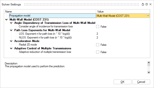
Solver Settings

Analysis > Options > Solver Settings

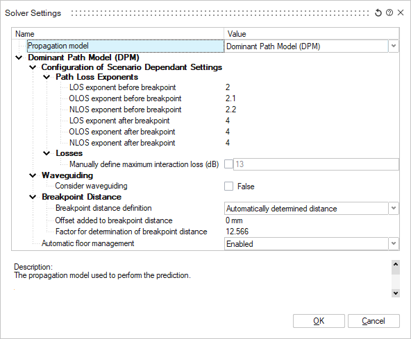
The Solver Settings dialog is used to specify the propagation model used for the simulation as well as settings related to the chosen model.

Dominant Path Model (DPM)

The dominant path model (DPM) determines the dominant path between the transmitter and each receiver pixel. So the computation time compared to ray-tracing is significantly reduced and the accuracy is nearly identical to ray-tracing.

Ray-optical propagation models are still time-consuming – even with accelerations like preprocessing. And what is even more important, they rely on an accurate vector database. Small errors in the database influence the accuracy of the prediction. On the other hand, empirical models are rely on dedicated propagation effects like the over-rooftop propagation (for example, the direct ray COST 231).

A comparison of prediction results computed with three types of prediction models is presented in the following figure with Empirical COST 231 (on the left), SRT (in the middle) and indoor dominant path (to the right):

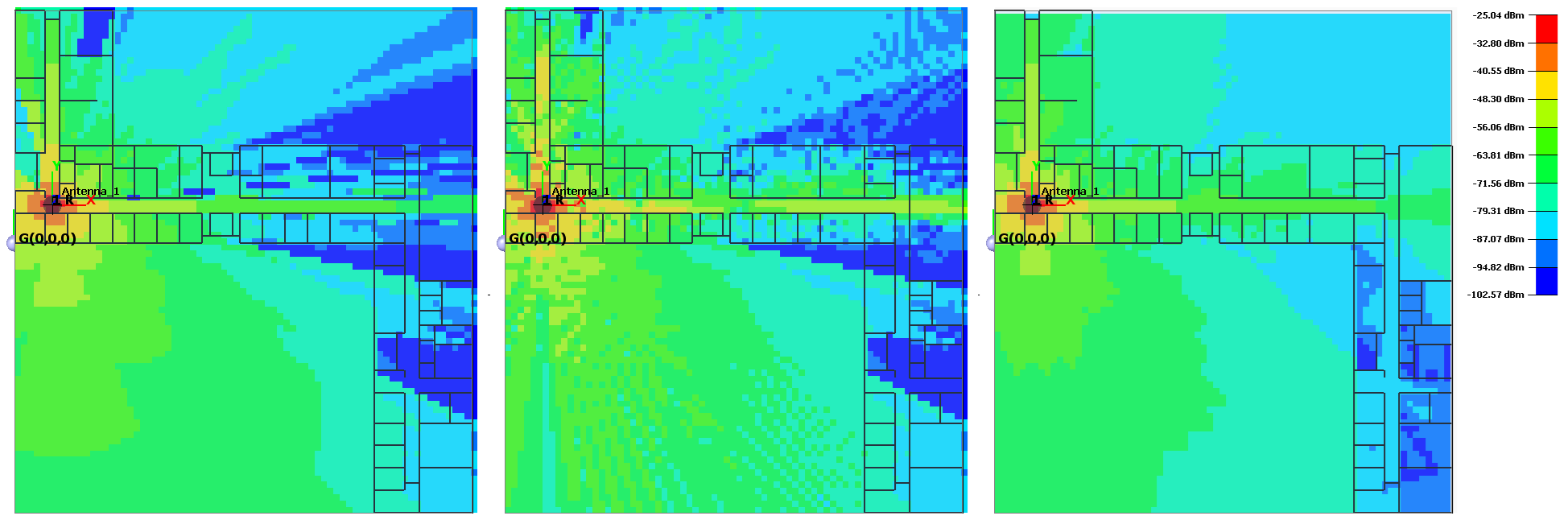
Analyzing typical propagation scenarios shows that in most cases one propagation path contributes more than 90% of the total energy. The dominant path model (DPM) determines exactly this dominant path between the transmitter and each receiver pixel. So the computation time compared to ray-tracing is significantly reduced and the accuracy is nearly identical to ray-tracing.

Empirical models (like COST 231) consider only the direct path between a transmitter and a receiver pixel. Ray tracing models (like IRT) determine numerous paths. DPM determines only the most relevant path, which leads to short computation times.

Comparison of different approaches (COST 231 on the left, ray-tracing in the middle and DPM to the right):

Advantages of the Dominant Path Model

As a consequence of the properties and restrictions of the available prediction models mentioned above, the dominant path prediction model (DPM) has been developed. The main characteristics of this model are:

The dependency on the accuracy of the vector database is reduced (compared to ray-tracing).
Only the most important propagation path is considered, because this path delivers the main part of the energy.
No time-consuming preprocessing is required (in contrast to IRT).
Short computation times.
Accuracy reaches or exceeds the accuracy of ray-optical models.

Typical Application of the Dominant Path Model

As the dominant path model does not require a preprocessing of the building vector database, it is ideally suited for large indoor areas. Additionally the approach to compute only the dominate ray emphasizes this operational area. The model does not compute the complete channel impulse response, as a result, if you are interested in the channel impulse response, the delay spread or the angular spread, a ray-tracing model is recommended. The DPM is the ideal approach to compute coverage predictions in large multi-story indoor environments.

Algorithm of the Dominant Path Model

The DPM determines the dominant path between transmitter and each receiver pixel. The computation of the path loss is based on the following equation:

L = 20 \log (\frac{4 π}{λ}) + 10 p \log (l) + \sum_{i = 1}^{n} f (φ, i) + \sum_{j = 1}^{m} t_{j} - Ω - g_{t}

where L is the path loss computed for a specific receiver location. The following parameters are considered by the model:

Distance from transmitter to receiver (l)
Path loss exponent (p)
Wave length (λ)
Individual interaction losses due to diffractions (f)
Individual transmission losses of all penetrations (t)
Empirically determined loss reduction due to wave guiding (Ω)
Gain of transmitting antenna (g_t)

As described above, l is length of the path between transmitter and current receiver location. p is the path loss exponent. The value of p depends on the current propagation situation. In buildings with a lot of furniture (which is not included in the vector modeling) p = 2.3 is suggested, whereas in empty buildings p = 2.0 is reasonable. The function f yields the loss (in dB) which is caused by diffractions. The diffraction losses are accumulated along one propagation path. Reflections and scattering are included empirically. For the consideration of reflections (and scattering), an empirically determined wave guiding factor is introduced.

This wave guiding factor takes into account, that a wave propagating in a long close corridor will be reflected on the walls leading to less attenuation compared to free space. Thus, wave guiding effects can be expressed as an additional gain in dB. The transmission (penetration) losses are also accumulated along the one propagation path. The directional gain of the antenna (in direction of the propagation path) is also considered.

Configuration of the Dominant Path Model

Path Loss Exponents

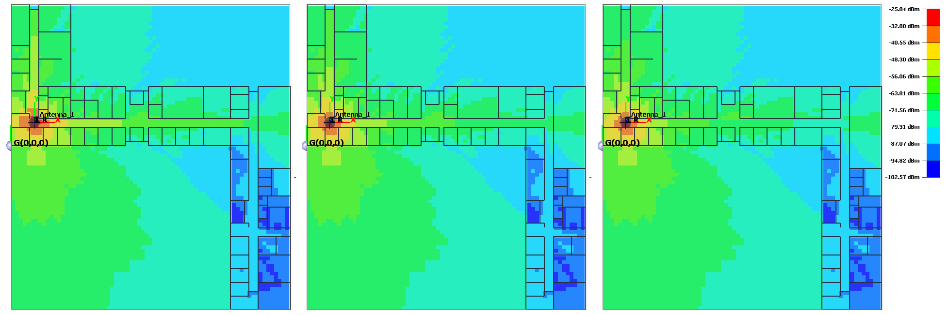
The path loss exponents influence the propagation result computed by the DPM significantly. The path loss exponents describe the attenuation with distance. A higher path loss exponent leads to a higher attenuation in same distance.

Comparison of three different predictions using different path loss values. LOS exponent 2.0 (on the left), LOS exponent 2.3 (in the middle) and LOS exponent 2.6 (to the right):

The following table shows recommended path loss exponents. The more objects that are missing in the vector database, the higher the path loss exponent should be.

Recommended path loss exponents:


Environment	Empty buildings	Filled buildings
LOS	2.0	2.1
OLOS	2.1	2.3
NLOS	2.2	2.5

Environment Empty buildings Filled buildings

Losses

Each change in the direction of propagation due to an interaction (diffraction, transmission/penetration) along a propagation path causes an additional attenuation. The maximum attenuation can be defined. The effective interaction loss depends on the angle of the diffraction.

It is recommended to select Auto. The transmitter frequency will then be taken into account in the calculation of maximum interaction loss.

Waveguiding effects

As mentioned before, the DPM includes waveguiding effects to achieve accurate results. Two parameters are available to configure the wave guiding module. The first parameter is used to define the maximum distance to walls to be included in the determination of the wave guiding factor. With the second parameter the weight of the wave guiding effects in the computation of the path loss is defined ( 1.0 is suggested. Values below 1.0 reduce the influence of the wave guiding factor and values above 1.0 increase it). In typical scenarios the wave guiding effects can be turned off, this reduces the prediction time.

Breakpoint distance

The breakpoint distance describes the distance from the transmitter when destructive superposition of the direct ray and the ground reflected ray occurs. Because of that the attenuation is much higher and thus larger path loss exponents are often used. The default distance for the breakpoint distance in indoor environments is 500 m.

Standard Ray Tracing (SRT)

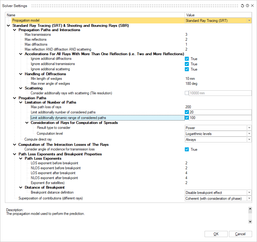
The standard ray-tracing model (SRT) performs a rigorous 3D ray-tracing prediction which results in a very high accuracy, but it is computationally expensive.

Deterministic models are used to simulate the propagation of radio waves physically. Therefore, the effect of the environment on the propagation parameters can be taken into account more accurately. Another advantage is that deterministic models make it possible to predict several propagation parameters. For example, the path loss, impulse response and angle-of-arrival can be predicted at the same time.

The following image shows the principle of ray optical models:

As smaller wavelengths (higher frequencies) are considered, the wave propagation becomes similar to the propagation of light. Therefore a radio ray is assumed to propagate along a straight line influenced only by refraction, reflection, diffraction or scattering which is the concept of geometrical optics ( GO). The criterion taken into account for this modelling approach is that the wavelength should be much smaller in comparison to the extension of the considered obstacles, for example, the walls of a building. At the frequencies used for mobile communication networks this criterion is also inside buildings sufficiently fulfilled.

There are two different basic approaches for the determination of the ray paths between transmitter and receiver in the geometrical optics technique:

ray-tracing
ray launching

The standard ray-tracing model (SRT) performs a rigorous 3D ray-tracing prediction which results in high accuracy. Due to the determination of the individual paths, the computational effort is large. Therefore several acceleration techniques both with and without loss of accuracy are developed and integrated in this rigorous 3D approach.

This model has a long computation time, because only small parts of the prediction are pre-processed and every propagation path is analytically determined.

Propagation Paths

Each transmission through a wall, each reflection at a wall and each diffraction at an edge counts as an interaction. The computed propagation paths can be limited within the propagation model settings. The value Max defines the maximum number of interactions that are allowed for each propagation path. The appropriate value depends on the building structure. If, for example, the building has a corridor that runs around a corner three times, then it would be better to compute more interactions, because multiple diffractions are needed to reach all prediction pixels. The same occurs if a building has a structure where the rays have to pass many walls to reach every point of the building, because then more transmissions are needed. The only constraint is that the computation time naturally increases if more interactions are computed. On the other hand, if too less interactions are computed, the accuracy decreases. In this case additionally more prediction pixels might not be reached by the SRT prediction, which leads to the need to compute those pixels with an empirical model which will decrease the accuracy even more. As a basic rule, an appropriate setting for the maximum value would be 2 – 4, depending on the building structure.

Computation of Each Ray's Contribution

For the computation of the rays, not only the free space loss has to be considered but also the loss due to the transmissions, reflections and (multiple) diffraction. This is either done using a physical deterministic model or using an empirical model.

Note: This does only affect the determination of the transmission, reflection and diffraction coefficients. The prediction itself always remains a deterministic one (the same rays are taken into account).

The deterministic model uses Fresnel equations for the determination of the reflection and transmission loss and the GTD / UTD for the determination of the diffraction loss. This model has a slightly longer computation time and uses three physical material parameters (permittivity, permeability and conductivity). When using GTD / UTD and Fresnel coefficients arbitrary linear polarizations (between +90° and –90°) or circular polarization can be considered for the transmitters. The empirical model uses five empirical material parameters (minimum loss of incident ray, maximum loss of incident ray, loss of diffracted ray, reflection loss, transmission loss). For correction purposes or for the adaptation to measurements, an offset to those material parameters can be specified. Here with the empirical model has the advantage that the needed material properties are easier to obtain than the physical parameters required for the deterministic model. Also the parameters of the empirical model can more easily be calibrated with measurements. It is therefore easier to achieve a high accuracy with the empirical model.

The effect of bookshelves and cupboards covering considerable parts of walls is taken into account by including an additional loss of the wall's penetration (transmission) loss. An additional loss of 3 dB was observed to be appropriate. This additional loss is introduced in context of walls covered by bookshelves, cupboards or other large pieces of furniture. Furthermore, it was found necessary to set an empirical limit for the wall transmission loss which otherwise becomes very high when the angle of incidence is large. The following interaction types exist:

Specular Reflection

The specular reflection phenomena is the mechanism by which a ray is reflected at an angle equal to the incidence angle. The reflected wave fields are related to the incident wave fields through a reflection coefficient which is a matrix when the full polarimetric description of the wave field is taken into account.

The most common expression for the reflection is the Fresnel reflection coefficient which is valid for an infinite boundary between two mediums, for example, air and concrete. The Fresnel reflection coefficient depends on the incident wave field and upon the permittivity and conductivity of each medium. The application of the Fresnel reflection coefficient formulas is very popular.

Diffraction

The diffraction process in ray theory is the propagation phenomena which explain the transition from the lit region to the shadow regions behind the corner or over the rooftops. Diffraction by a single wedge can be solved in various ways: empirical formulas, perfectly absorbing wedge, geometrical theory of diffraction (GTD) or uniform theory of diffraction (UTD). The advantages and disadvantages of using either one formulation is difficult to address since it may not be independent on the environments under investigation. Indeed, reasonable results are possible with each formulation. The various expressions differs mainly from the approximations being made on the surface boundaries of the wedge considered. One major difficulty is to express and use the proper boundaries in the derivation of the diffraction formulas. Another problem is the existence of wedges in real environments: the complexity of a real building corner or of the building’s roof illustrates the modelling difficulties.

Despite these difficulties, however, diffraction around a corner or over rooftop are commonly modelled using the heuristic UTD formulas since they are well behaved in the lit/shadow transition region, and account for the polarization as well as for the wedge material. Therefore these formulas are also used to calculate the diffraction coefficient.

Multiple Diffraction

For the case of multiple diffraction the complexity increases dramatically. One method frequently applied to multiple diffraction problems is the UTD. The main problem with straightforward applications of the UTD is, that in many cases one edge is in the transition zones of the previous edges. Strictly speaking this forbids the application of ray techniques, but in the spirit of the UTD the principle of local illumination of an edge should be valid. At least within some approximate degrees, a solution can be obtained which is quite accurate in most cases of practical interest.

The key point in the theory is to include slope diffraction, which is usually neglected as a higher order term in an asymptotic expansion, but in the transition zone diffraction the term is of the same order as the ordinary amplitude diffraction terms. Additionally there is an empirical diffraction model available which can easily be calibrated with measurements.

Scattering

Rough surfaces and finite surfaces (surfaces with small extension in comparison to the wavelength) scatter the incident energy in all directions with a radiation diagram that depends on the roughness and size of the surface or volume. The dispersion of energy through scattering means a decrease of the energy reflected in specular direction. This simple view leads to account for the scattering process by only decreasing the reflection coefficient. The reflection coefficient is decreased by multiplying it with a factor smaller than one where this factor is exponentially dependent on the standard deviation of the surface roughness according to the Rayleigh theory. This description does not take into account the true dispersion of radio energy in various directions, but accounts for the reduction of energy in the specular direction due to the diffuse components scattered in all other directions.

Penetration and absorption

Penetration loss due to building walls have been investigated and found to be dependent on the particular system. Absorption due to trees or the body absorption are also propagation mechanisms difficult to quantify with precision. Therefore in the radio network planning process adequate margins should be considered to ensure overall coverage. Another absorption mechanism is the one due to atmospheric effects. These effects are usually neglected in propagation models for mobile communication applications at radio frequencies but are important when higher frequencies (for example 60 GHz) are used.

Propagation Paths and Interactions

The Propagation paths and interactions group allows to specify the number of interactions that should be considered for the determination of ray paths between transmitter and receiver including the maximum number of reflections, diffractions and scattering.

To accelerate the prediction, additional diffractions and transmissions can be ignored for all rays with more than one reflection. The minimum length of wedges where diffractions can occur can be specified in meters. In case the simulation database contains ground objects (topography in vector format), interaction at those objects can optionally be considered. Diffuse scattering in indoor scenarios can play an important role, especially for determining the actual temporal and angular dispersion of the radio channel.

The WinProp SRT model was extended to consider the scattering on building walls and other objects. For this purpose the scattering can be activated in the model settings by enabling the option “Consider additionally rays with scattering”. As the scattering increases the overall number of rays significantly, there is a limitation of one scattering per ray. Furthermore, the surface roughnesses of the corresponding materials need to be defined.

For the scattering in the SRT model, tiles as defined in the dialog are considered. The scattered contribution is weighted with the size of the scattering area (tile). Accordingly the resulting scattered power from the whole object is for large distances independent of the tile size. For small distances there is an impact due to the modified scattering angles which depend on the tile size. The tile size for ground scattering can be chosen different from that on buildings.

Propagation Paths

This option allows the limitation of the number of paths per pixel with the following options: maximum path loss of rays, maximum number of paths or dynamic range of paths.

Propagation Paths - Direct Ray

The direct ray can be computed always, despite the number of transmissions specified in the first section.

Computation of interaction losses of the rays

For the computation of the rays, not only the free space loss has to be considered but also the loss due to the transmissions, reflections and (multiple) diffraction. Optionally the interaction losses of the rays can be determined considering the angle of incidence for the calculation of the transmission loss.

Path Loss Exponent for ray-optical models

Exponent for distance-dependent path loss.

Superposition of contributions (different rays)

Superposition of contributions of different rays can be done either incoherent (without consideration of the phases) or coherent (with consideration of the phases).

3D Shooting and Bouncing Rays (SBR)

The Shooting and Bouncing Rays (SBR) method performs a rigorous 3D ray-launching prediction which results in a high accuracy, but it can be computationally expensive. Deterministic models are used to simulate the propagation of radio waves physically. Therefore, the effect of the environment on the propagation parameters can be taken into account more accurately.

Another advantage is that deterministic models make it possible to predict several propagation parameters. For example, the path loss, impulse response and angle-of-arrival can be predicted at the same time. Since both the SBR and SRT methods are deterministic models, the description and settings used are similar. In addition to those of SRT, the SBR method has the following settings:

Ray density

Since the SBR method starts by launching rays from the antenna, and, contrary to SRT, does not guarantee that every possible path will be found, the ray density parameters are important.

The Max ray tube side width/height, i.e., the width and the height of the small outgoing wave front of the ray tube, determines the minimum geometrical detail size that will affect the rays. Ray tubes are split to ensure that any ray tube cross section at an intersection with an object will not exceed the square of this value.

The Ray length to first split is the distance at which the splitting may commence. This length, in combination with the maximum tube side width and height, determines the number of rays that will be launched initially. For instance, if this length is 1 m and the maximum tube width × height is 10×10 cm², then 1257 rays will be launched to cover the 1-meter sphere with area 4π m².

Figure 1. The concept of ray splitting to achieve proper ray density at interactions with objects.

In Figure 1, the orange rays are the original rays. An intersection algorithm determines where interactions may occur. This algorithm ensures that any object larger than the minimum geometrical detail size (see above) will be found, even if it might be between orange rays in the figure. Geometry elements smaller than the maximum ray tube side width and height are not ignored. You can still get interactions at those, but the algorithm cannot guarantee that those are illuminated by at least a single ray. At each interaction point the area of the ray cross section is computed. If this exceeds the user set maximum, the ray segment is repeated with multiple, split rays, to ensure that the maximum ray tube width and height are not exceeded at the interaction. The original ray (dotted in the Figure 1) is discarded and replaced by the split rays (green rays in Figure 1). The directions of the split rays are computed such that the ray cross sections cover the whole area of the original ray tube’s front.

Note: Ray length to first split is ideally set such that it is at least the distance between the transmitter and the closest geometry (any geometry in the scenario, but avoid choosing a distance close to zero if the transmitter is mounted on an object).

If the distance is set too large, the ray density close to the transmitter becomes unnecessarily high, and objects close to the transmitter, are hit by many more rays than needed, which slows down the computation. The distance to first split will be reduced automatically if needed to ensure that no more than 50 million rays be launched from the transmitter.

Note: Max ray tube side width/height should always be smaller than the discretization of the result pixels to reduce the chance that a result pixel will not receive any rays.

The Gain adaptation determines to what extend a higher ray density will be used in directions with higher antenna gain. Options are Off, Low, Medium, High.

Low

If the antenna gain for a direction is higher than MaxGain - 1 * 6dB the density will be increased for that direction by a factor of 2 (side length).

Medium

If the antenna gain for a direction is higher than MaxGain - 2 * 6dB the density will be increased for that direction by a factor of 2 (side length).

If the antenna gain for a direction is higher than MaxGain - 1 * 6dB the density will be increased for that direction by a factor of 4 (side length).

High

If the antenna gain for a direction is higher than MaxGain - 3 * 6dB the density will be increased for that direction by a factor of 2 (side length).

If the antenna gain for a direction is higher than MaxGain - 2 * 6dB the density will be increased for that direction by a factor of 4 (side length).

If the antenna gain for a direction is higher than MaxGain - 1 * 6dB the density will be increased for that direction by a factor of 8 (side length).

Scattered rays per impact determines how many new rays are spawned at each scattering interaction. If the physics of the scattering predicts a lobe in a certain direction, then the density of new rays in that lobe will automatically be higher than in other directions.

Diffracted rays per impact determines how many new rays are created at each diffraction interaction.

Multi-Wall Model (COST 231)

The multi-wall model gives the path loss as the free space loss added with losses introduced by the walls and floors penetrated by the direct path between transmitter and receiver.

It has been observed that the total floor loss is a function of the number of the penetrated floors. This characteristic is taken into account by introducing an additional empirical correction factor.

The individual penetration losses for the walls (depending on their material parameters) are considered for the prediction of the path loss. Therefore, the multi-wall model can be expressed as follows:

l_{M W} = l_{F S} + l_{c} + k_{f} l_{f} + \sum_{i = 1}^{N} k_{w i} l_{w i}

where:

l_FS: Free space loss between transmitter and receiver
l_c: Constant loss
k_wi: Number of penetrated walls of type i
k_f: Number of penetrated floors
l_wi: Loss of wall type i
l_f: Loss between adjacent floors
N: Number of different wall types

The constant loss in the equation above is a term which results when wall losses are determined from measurement results by using multiple linear regression. Normally it is close to zero. The third summand in the equation represents the total wall loss as a sum of the walls between transmitter and receiver. For practical reasons the individual wall loss of the intersected walls is considered.

It is important to notice that the loss factors in the formula express not physical wall losses but model coefficients which are optimized with the measured path loss data. Consequently, the loss factors implicitly include the effect of furniture. However, wave guiding effects are not considered with this model, thus the accuracy is moderate. On the other hand, this model has a low dependency on the database accuracy and because of the simple approach a very short computation time. Therefore, no preprocessing of the building data is needed for the computation of the prediction and no settings have to be adapted for this prediction model.