Phase 2: Shell Flat Plate

The objective is to create linear static models for shell models.

Launch HyperMesh and Set the OptiStruct User Profile

Launch HyperMesh.
The User Profile dialog opens.
Select OptiStruct and click OK.
This loads the user profile. It includes the appropriate template, macro menu, and import reader, paring down the functionality of HyperMesh to what is relevant for generating models for OptiStruct.

Import the Model

Click File > Import > Solver Deck.
An Import tab is added to your tab menu.
For the File type, select OptiStruct.
Select the Files icon .
A Select OptiStruct file browser opens.
Select the Flat_plate.fem file you saved to your working directory.
Click Open.
Click Import, then click Close to close the Import tab.

Set Up the Model

Create Material Properties

Create the material and property collectors before creating the component collectors.

In the Model Browser, right-click and select Create > Material.
A default MATUSR material displays in the Entity Editor.
For Name, enter MATUSR.
Activate USUBID and enter a value of 1.
This allows you to define different types of material properties. This value corresponds to the idu variable in the user subroutine.
Activate NDEPVAR and enter a value of 1.
Number of user-defined state variables. This value corresponds to the nstate(*) variable in the user subroutine.

Tip: Since there are no thermal loads in this model, leave the box in front of EXPAN unchecked. If the EXPAN parameter is defined, the final one (ISO), final three (ORTHO), or final six (ANISO) PROPi values are used as the corresponding thermal expansion coefficients. The default is ISO.
Activate GROUP and enter GRP.

User-defined group specified on the group argument of the LOADLIB entry. This field is used to identify the LOADLIB entry to load the corresponding .dll or .so file.
For MATUSR_PROPERTY, enter 2.
It will generate a table, as shown below.

Figure 1. MATUSR Property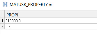
In the first row [E] Young’s modulus, enter 2.1E+05.
In the second row [Nu] Poisson’s ratio, enter 0.3.

Figure 2. MATUSR Entity Editor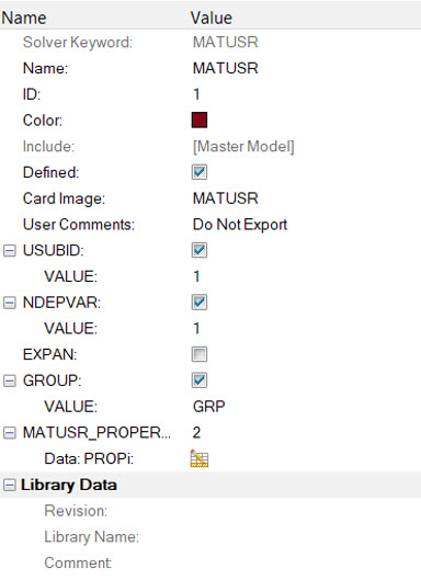

Define User Material

In this step, you will setup the smatusr subroutine to accept the two material properties (E and NU) and assemble the constitutive material model matrix for use in the analysis. For more information, refer to User-Defined Structural Material in the User Guide.

Important:

While writing Fortran code you must follow the guidelines and syntax properly.
SMATUSR subroutine is only used when the problem is linear or SMDISP.

Warning: Do not change name and arguments of subroutine function.

Navigate to the examples folder and open the umat_barebones.F Fortran file.

This provides you with some placeholder code for usermaterial subroutine (which is not relevant for this tutorial), and a barebones initial smatusr subroutine. The umat_barebones.F file should contain the smatusr barebones subroutine definition, as shown below.

subroutine smatusr(  idu, nprop, prop, ndi, nshear, ntens,
     $                        smat, ieuid )
      !DEC$ ATTRIBUTES DLLEXPORT :: smatusr
      implicit none
c----------------
c --- Arguments 
c----------------      
      integer igroup, nprop,idu, ieuid
      integer ndi, nshear, ntens     
      double precision prop(nprop), smat (*)
c---------------------      
c --- Local variables
c--------------------- 
      integer i,j, iii, k
      double precision pe, pnu, pmu, rlamda
      double precision cjac(ntens,ntens

Important: It is important that the subroutine is named smatusr.

The variables, parameters, and arguments used in the subroutine are explained below.

!DEC$ ATTRIBUTES DLLEXPORT

This attribute directive option DLLEXPORT define a dynamic-link library's interface for processes that use them. DLLEXPORT specifies that procedures or data are being exported to other applications or dynamic libraries.

implicit none

An IMPLICIT statement specifies a type and size for all user-defined names that begin with any letter, either a single letter or in a range of letters, appearing in the specification. An IMPLICIT statement does not change the type of the intrinsic functions. The implicit none statement is used to inhibit a very old feature of Fortran that by default treats all variables that start with the letters i, j, k, l, m and n as integers and all other variables as real arguments.

Arguments

Are declared, as shown above, according to the data type used in the code. Local variables are free to change, add, remove, and use according to your requirement.

The arguments passed to subroutine and its significance is mentioned in . For further reference, refer to User-Defined Structural Material.

Table 1. Description of the Argument in the subroutine
Argument	Type	Input / Output	Description
`idu`	integer	Input	(Optional) This is defined via the `USUBID` parameter on the MATUSR Bulk Data Entry. This argument can be used to define and choose between different types of materials within the same user-subroutine.
`props`	double (table)	Input	This table contains all the user-defined material property information from the `PROPERTY` continuation line of the MATUSR entry.
`nprops`	Integer	Input	This is the total number of material properties defined on the `PROPERTY` continuation line of the MATUSR entry.
`ndi`	Integer	Input	The number of normal stress components (3 for solid elements, 2 for shell elements).
`nshear`	Integer	Input	The number of shear stress components (3 for solid elements, 1 for shell elements).
`ntens`	Integer	Input	The number of tensor components (`ntens` = `ndi` + `nshear`).
`ieuid`	integer	Input	Element ID. This subroutine is called for every integration point for every element.
`smat`	Double (table)	Output	1D array (21 terms). This is the symmetric part of `cdev`. These are calculated during the solution and are output to OptiStruct to form the stiffness matrix.

Here the input material properties (PROPi) passed using the MATUSR card are assigned to local variables.
```
      if(nprop.lt.2)then
         write(*,*)'*** ERROR in smatusr: nprop.lt.2 ***',nprop
      endif

      pe = prop(1)
      pnu = prop(2)
      pmu = 0.5d0*pe/(1.0d0+pnu)
      rlambda =(pe*pnu)/((1.0d0+pnu)*(1.0d0-2*pnu))
```
1. For this model, the user-defined input material properties (PROPi) should not be less than 2. If less than 2, an error is issued.
2. The properties defined via PROPi on MATUSR are available in the subroutine for use through the prop(i) variables. So pe is assigned as Young’s modulus and the pnu is assigned as Poisson’s ratio.
  
  Subsequently, Lame’ constants are calculated [lambda] and [mu]. In continuum mechanics, Lamé parameters are two material-dependent quantities denoted by $λ$ and $μ$ that arise in strain-stress relationships. The Lamé parameters are dependent on the elasticity modulus E and the Poisson’s ratio $v$ . In general, $λ$ and $μ$ are individually referred to as first Lamé parameter and second Lamé parameter, respectively.
Next, you will need to initialize and formulate Jacobian matrix (cjac matrix) of the constitutive model which is the second derivative of stress to second derivative of strain.
```
do i=1,ntens
         do j=1,ntens
             cjac(i,j)=0
         enddo
         enddo
         do i=1,ndi
         do j=1,ndi
             cjac(i,j)=rlambda
         enddo
         enddo
         do i=1,ndi
             cjac(i,i)=cjac(i,i)+2.0d0*pmu
         enddo
	  
         do i=ndi+1,ntens
             cjac(i,i)=pmu
         enddo
```
1. For solid element, ntens = 6 (shown above), Jacobian matrix becomes cjac(6,6).
2. The cjac matrix is symmetric it is formulated by using Lamé parameters. The cjac matrix looks, as shown below.
  (1) $C j a c = [\begin{matrix} \frac{E}{1 - ν^{2}} & \frac{E ν}{1 - ν^{2}} & 0 \\ \frac{E ν}{1 - ν^{2}} & \frac{E}{1 - ν^{2}} & 0 \\ 0 & 0 & \frac{E (1 - ν)}{2 (1 - ν^{2})} \end{matrix}]$
  Where,
  
  E
  
  Young’s modulus
  
  $v$
  
  Poisson ratio
The Jacobian constitutive matrix is symmetric in this case, so the lower triangular matrix of 6 elements is stored in the smat array, as shown below.
```
iii=0 
      do j=1,ntens
      do i=j,ntens
            iii=iii+1 
            smat(iii) = cjac(i,j)
      enddo
      enddo

      return
      end
```
Note: The subroutine in the end returns the smat array to OptiStruct for further calculation.

Build External Libraries

To export external dynamic libraries from the Fortran code, in Windows or Linux, refer to Build External Libraries in the User Guide.

Note:

Save the .dll or .so file in the same repository so that it can be accessed easily when required.
The path of the dynamic library should be the same as mentioned in the LOADLIB card.
Verify that the library path, name, and extension are correct before solving the problem. Also, check that the library was compiled and linked properly with the problem.

Below is an example compilation of the umat.F file using the GNU Fortran Complier on Linux.

# rename the Fortran file for convenience
mv umat_barebones.F umat.F   # optional       
# compile and create object files
f95 -fPIC -c umat.F -o umat.o
# create the final shared library
ld -shared umat.o -o umat.so
# The shared library “umat.so” can now be used via LOADLIB entry in the OptiStruct run

Create PSHELL Property

In the Model Browser, right-click and select Create > Property.
A default PSHELL property displays in the Entity Editor
For Name, enter Pshell.
Click Color and select a color from the color palette.
For Card Image, select PSHELL and click Yes to confirm.
For Material, click Unspecified > Material.
For thickness, click T and enter 2.0.
In the Select Material dialog, select MATUSR.
Click OK.
The property of the MATUSR Shell has been created as PSHELL. Material information is linked to this property.

Figure 3. PSHELL element property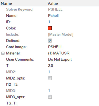

Link Material and Property to Existing Structure

After the material and property are defined, they will need to be linked to the structure.

In the Model Browser, click the component PLATE.
The Entity Editor opens.
For Property, click Unspecified > Property.
In the Select Property dialog, select Pshell and click OK.
The material MATUSR now is linked to the component PLATE.

Create SPC Load Collector

Two load collectors will be created in this step.

In the Model Browser, right-click and select Create > Load Collector.
A default load collector template displays in the Entity Editor.
For Name, enter spc.
Click Color and select a color from the color palette.
A new load collector, spc is created.
For Name, enter force for the second load collector.
Click Color and select a color from the color palette.
A new load collector, force is created.

Figure 4. Create the Load Collectors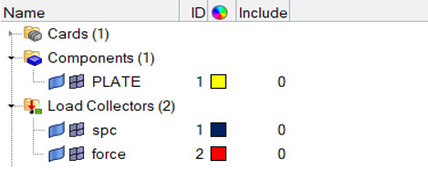

Create Constraints

Here you will create constraints at one end of cylinder.

In the Model Browser, right-click on spc and select Make Current.
Click BCs > Create > Constraints.
The Constraints panel opens.
Click the entity selection switch and select nodes from the menu.
Select the edges by toggle down and select the edge at one end.
The nodes have been selected.

Figure 5. Create constraints at one end of plate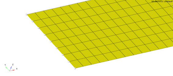
Activate/constrain all dof.

Note: DOFs with a check will be constrained.
Select create.
Constraints are created. Constraint symbols (triangles) appear in the graphics area at the selected nodes. The numbers are written beside the constraint symbol, indicating the dof constrained.
In the size field, enter 1.0.

Note: The size of the constraint symbols in the graphics area changes.
Click return to go to the main menu.

Apply Force

This step shows how to apply force on the other end of the cylinder.

In the Model Browser, right-click on force and select Make Current.
Click BCs > Create > Forces.
The Force panel opens.
Click the entity selection switch and select nodes from the menu.
Select the edges by toggle down and select the nodes at opposite end.
For coordinates, select global system, then select Y-axis.
For magnitude =, enter 10.
For load types = select FORCE.

Figure 6. Force magnitude and vector selection for selected nodes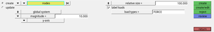
In the relative size field, enter 100.0.

Note: The size of the constraint symbols in the graphics area changes.
Click return to go to the main menu.

Create Linear Load Step

Here you will create an OptiStruct subcase (also referred to as a loadstep).

In the Model Browser, right-click and select Create > Load Step.
A default load step template is now displayed in the Entity Editor.
For Name, enter Linear.
Expand Analysis type and select Linear Static.
For SPC, click Unspecified > Loadcol.

Figure 7. Linear static loadstep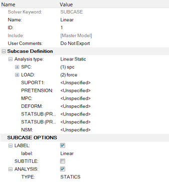
In the Select Loadcol dialog, select spc and click OK.
For LOAD, click Unspecified > Loadcol.
In the Select Loadcol dialog, select force and click OK.

Select the Shared Library

From the Analysis page, select Control Cards.
For control cards, select LOADLIB.

Figure 8. LOADLIB card assign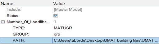
For Number_Of_Loadlibs, enter 1.
For TYPE, select MATUSR.
For GROUP, enter grp.
Enter the location of the .dll or .so file, as shown above.

Submit the Job

From the Analysis page, click the OptiStruct panel.

Figure 9. Accessing the OptiStruct Panel
Click save as.
In the Save As dialog, specify location to write the OptiStruct model file and enter Flat_plate.fem for filename.
For OptiStruct input decks, .fem is the recommended extension.
Click Save.
The input file field displays the filename and location specified in the Save As dialog.
Set the export options toggle to all.
Set the run options toggle to analysis.
Set the memory options toggle to memory default.
Click OptiStruct to launch the OptiStruct job.

If the job is successful, new results files should be in the directory where the Flat_plate.fem was written. The Flat_plate.out file is a good place to look for error messages that could help debug the input deck if any errors are present.

The default files written to the directory are:

Flat_plate.html: HTML report of the analysis, providing a summary of the problem formulation and the analysis results.
Flat_plate.out: OptiStruct output file containing specific information on the file setup, the setup of your optimization problem, estimates for the amount of RAM and disk space required for the run, information for each of the optimization iterations, and compute time information. Review this file for warnings and errors.
Flat_plate.h3d: HyperView binary results file.
Flat_plate.res: HyperMesh binary results file.
Flat_plate.stat: Summary, providing CPU information for each step during analysis process.

View the Results

Displacement and Stress results are output from OptiStruct for linear static analyses by default. The following steps describe how to view those results in HyperView.

View a Contour Plot of Displacements and Stresses

When the message 'ANALYSIS COMPLETED' is received in the Solver View window, click Results.
HyperView is launched and the results are loaded.
Set the Animation Mode to Linear .
Click the Contour toolbar icon .
Select the displacement. Select the displayed component click Apply.
Plot the result.
Click the Contour toolbar icon .
Select the first pull-down menu below Result type: and select Element Stresses (2D & 3D) (t).
Select the second pull-down menu below Result type: and select vonMises.
For Averaging method, select Simple and click Apply.

Figure 10. Contour selecting the Result type as Elemental Stresses and averaging method as Simple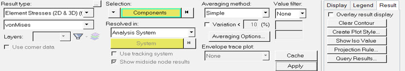

There is a good match between the two material modeling approaches (MAT1 versus MATUSR).

Figure 11. Isometric view of results of Plate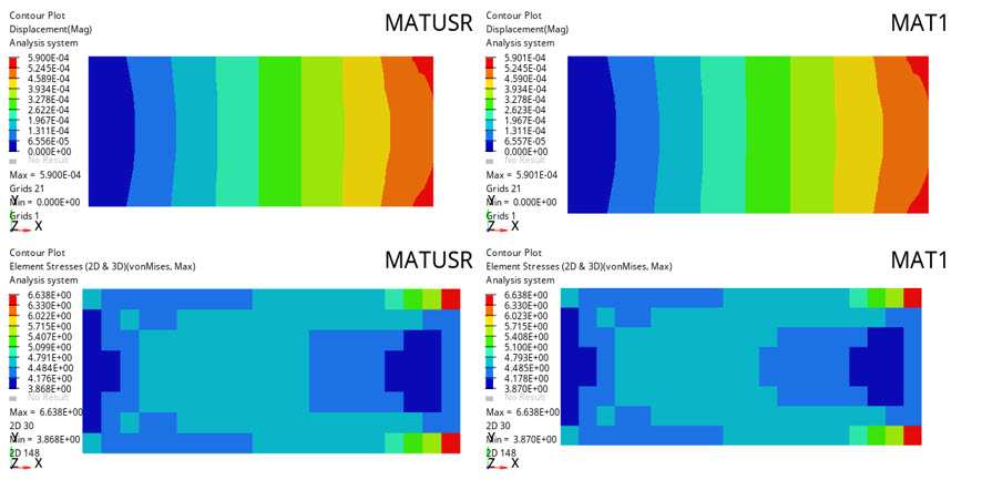
Click File > Exit to leave HyperView.