OS-T: 1000 Linear Static Analysis of a Plate with a Hole
This tutorial demonstrates the creation of finite elements on a given CAD geometry of a plate with a hole. Further, application of boundary conditions and a finite element analysis of the problem are explained. Post-processing tools are used in HyperView to determine deformation and stress characteristics of the loaded plate.
Launch HyperMesh and Set the OptiStruct User Profile
-
Launch HyperMesh.
The User Profile dialog opens.
-
Select OptiStruct and click
OK.
This loads the user profile. It includes the appropriate template, macro menu, and import reader, paring down the functionality of HyperMesh to what is relevant for generating models for OptiStruct.
Open the Model
- Click .
- Select the plate_hole.hm file you saved to your working directory.
-
Click Open.
The plate_hole.hm database is loaded into the current HyperMesh session, replacing any existing data.
Set Up the Model
Create the Material
-
In the Model Browser, right-click and select from the context menu.
A default material displays in the Entity Editor.
- For Name, enter steel.
- Set Card Image to MAT1.
-
Enter the material values next to the corresponding fields.
- For E (Young's Modulus), enter 2.1E+05.
- For NU, (Poisson's Ratio), enter 0.3.
- For RHO (Mass Density), leave it undefined since only a static analysis is performed.
Figure 1. Material Property Values for steel 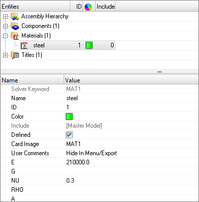
A new material, steel, has been created. The material uses OptiStruct's linear isotropic material model, MAT1. - Click Close.
Create the Property
-
In the Model Browser, right-click and select from the context menu.
A default property displays in the Entity Editor.
- For Name, enter plate_hole.
- Set Card Image to PSHELL.
-
Enter the property values next to the corresponding fields.
An empty Value field indicates that it is turned off. To edit these properties, click on the blank Value fields next to them and enter the required values.
- For Material, click . In the Select Material dialog, select steel and click OK.
- For T (thickness of the plate), enter 10.0.
Figure 2. Property Values for plate_hole 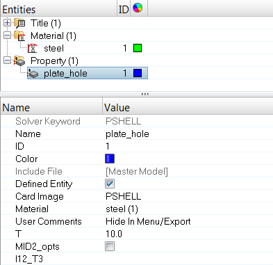
Update the plate_hole Component
-
In the Model Browser, click on the component plate_hole.
The component fields are displayed in the Entity Editor below.
-
For Property, click . In the Select Property dialog, select
plate_hole and click OK.
Figure 3. 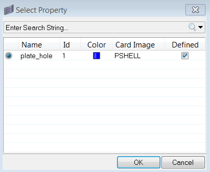
Apply Loads and Boundary Conditions
In the following steps, the model is constrained so that two opposing edges of the four external edges cannot move. The other two edges remain unconstrained. A total load of 1000N is applied at the edge of the hole in the positive z-direction.
Create Load Collectors
-
In the Model Browser, right-click and select from the context menu.
A default load collector displays in the Entity Editor.
- For Name, enter spcs.
- Click Color and select a color from the color palette.
-
Set Card Image to None and click
Close.
A new load collector, spcs is created.
Figure 4. Creating the spcs Load Collector 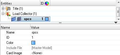
-
Create another load collector.
- For Name, enter forces.
- For Card Image, select None.
Create Constraints
-
In the Model Browser, Load Collectors folder, right-click
on spcs and select Make Current to
set spcs as the current load collector.
Figure 5. Setting spcs as the Current Load Collector 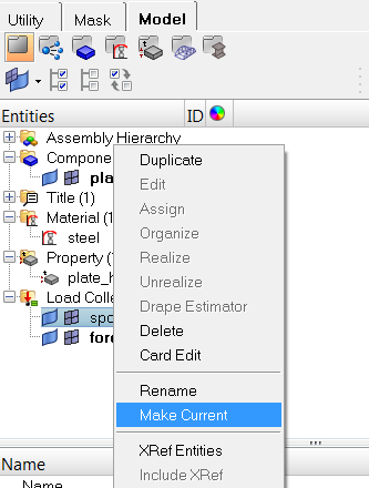
-
From the menu bar, click to open the Constraints panel.
Figure 6. Accessing the Constraints Panel 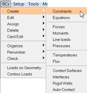
-
Make sure nodes is selected from the entity selection
switch.
Figure 7. Menu after Clicking on the Entity Selection Switch 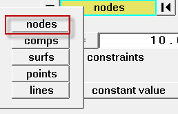
-
Hold Shift while clicking-and-dragging your mouse to
select the nodes on the two ends of the plate.
Figure 8. Nodes to Select for the Constraints 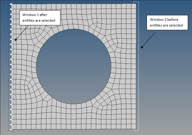
-
Constrain dof1, dof2,
dof3, dof4,
dof5, and dof6 and set all of
them to a value of 0.0.
- DOFs with a check will be constrained while DOFs without a check will be free.
- DOFs 1, 2, and 3 are x, y, and z translation degrees of freedom.
- DOFs 4, 5, and 6 are x, y, and z rotational degrees of freedom.
Figure 9. Constraining all Degrees of Freedom of the Selected Nodes 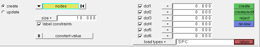
-
Click create.
Constraints are applied to the selected nodes.
- Click return to go back to the main menu.
Create Forces on the Nodes around the Hole
- In the Model Browser, set your current load collector to forces.
- From the menu bar, click to open the Forces panel.
-
Press Shift while left-clicking, then release your
mouse button to access selection options. Select Circle
Interior.
Figure 10. Choosing a Circular (Inside of Circle) Selection Window 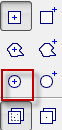
-
Hold Shift while clicking-and-dragging your mouse to
select the nodes around the hole.
Figure 11. Nodes Selected for the Application of Loads around the Hole 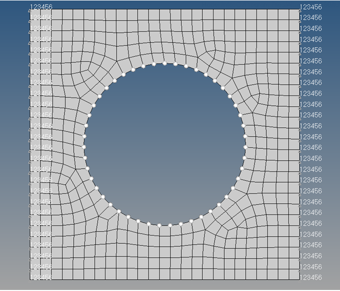
-
Define settings in the Forces panel.
- Set the coordinate system toggle to global system.
- Set the vector definition switch to constant vector.
- In the magnitude= field, enter 21.277 (that is 1000 divided by the number of nodes 47).
- Set the direction definition switch, below magnitude =, to z-axis.
Figure 12. Assign Direction and Magnitude to the Forces 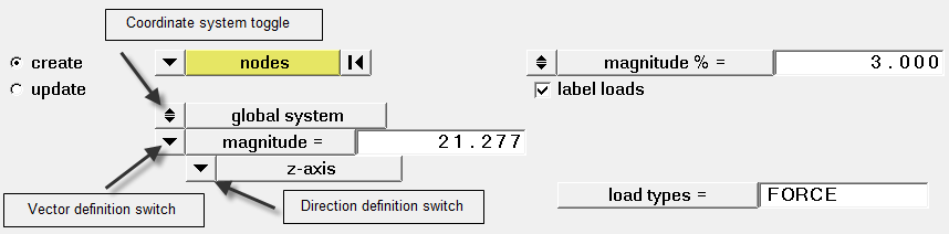
-
Click create.
Point forces, with the given magnitude in the z-direction, are applied to the selected nodes about the hole.
- Click return to go back to the main menu.
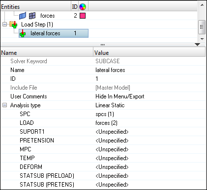
Create Load Steps
- In the Model Browser, right-click and select from the context menu.
- For Name, enter lateral forces.
- Set Analysis type to Linear Static.
-
Define SPC.
-
For SPC, click Unspecified >
 to open Advanced Selection.
- In the dialog, select spcs and click OK.
-
For SPC, click Unspecified >
- In Subcase Options, select .
-
For LOAD, click Unspecified > to open Advanced Selection.
- In the dialog, select forces and click OK.
An OptiStruct subcase has been created which references the constraints in the load collector spcs and the forces in the load collector forces.
Submit the Job
-
From the Analysis page, click the OptiStruct
panel.
Figure 14. Accessing the OptiStruct Panel 
- Click save as.
-
In the Save As dialog, specify location to write the
OptiStruct model file and enter
plate_hole for filename.
For OptiStruct input decks, .fem is the recommended extension.
-
Click Save.
The input file field displays the filename and location specified in the Save As dialog.
- Set the export options toggle to all.
- Set the run options toggle to analysis.
- Set the memory options toggle to memory default.
- Click OptiStruct to launch the OptiStruct job.
- plate_hole.html
- HTML report of the analysis, providing a summary of the problem formulation and the analysis results.
- plate_hole.out
- OptiStruct output file containing specific information on the file setup, the setup of your optimization problem, estimates for the amount of RAM and disk space required for the run, information for each of the optimization iterations, and compute time information. Review this file for warnings and errors.
- plate_hole.h3d
- HyperView binary results file.
- plate_hole.res
- HyperMesh binary results file.
- plate_hole.stat
- Summary, providing CPU information for each step during analysis process.
View the Results
Displacement and Stress results for linear static analyses are output from OptiStruct by default. The following steps describe how to view those results in HyperView.
HyperView is a complete post-processing and visualization environment for finite element analysis (FEA), multibody system simulation, video and engineering data.
View a Contour Plot of Stresses
-
From the OptiStruct panel, click HyperView.
HyperView is launched and the results are loaded. A message window appears to inform of the successful model and result files loading into HyperView.
-
On the Results toolbar, click
 to open the
Contour panel.
to open the
Contour panel.
-
Define settings in the Contour panel.
- Under Result type set the first first pull-down menu to Element Stresses (2D & 3D) (t) and set the second pull-down menu to vonMises.
- Set the Averaging method to None.
Figure 15. The Contour panel 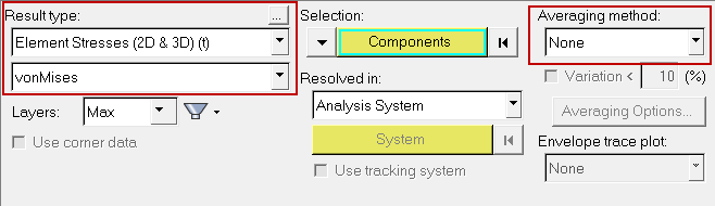
-
Click Apply.
A contoured image representing von Mises stresses should be visible. Each element in the model is assigned a legend color, indicating the von Mises stress value for that element, resulting from the applied loads and boundary conditions.
-
In the View Controls toolbar, click the XY Top Plane
View icon to change the view the model.
Figure 16. The von Mises Stress Plot for the Given Subcase 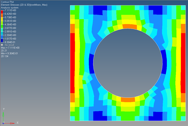
- What is the maximum von Mises stress value?
- At what location does the model have its maximum stress?
- Does this make sense based on the boundary conditions applied to the model?
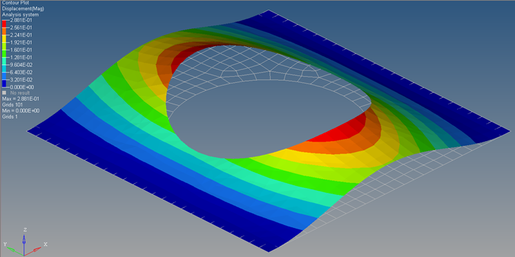
View a Contour Plot of Displacements
- Under Result type set the first first pull-down menu to Displacement (v) and set the second pull-down menu to Mag.
- Click Apply.
- What is the maximum Displacement value?
- At what location does the model have its maximum displacement?
- Does this make sense based on the boundary conditions applied to the model?
View the Deformed Shape
- In the View Controls toolbar, click the Isometric View icon to display the isometric view of the model.
-
Click the Deformed toolbar icon
 .
.
-
Define settings in the Deformed panel.
- Click Apply.