OS-T: 1080 Coupled Linear Heat Transfer/Structure Analysis
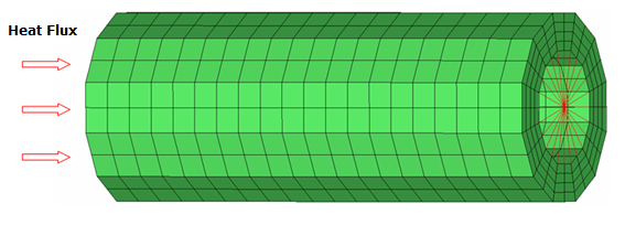
A coupled heat transfer/structure analysis on a steel pipe is performed in this tutorial.
As shown in Figure 1, the pipe is fixed on the ground at one end and the heat flux is applied on the other end.
Launch HyperMesh and Set the OptiStruct User Profile
-
Launch HyperMesh.
The User Profile dialog opens.
-
Select OptiStruct and click
OK.
This loads the user profile. It includes the appropriate template, macro menu, and import reader, paring down the functionality of HyperMesh to what is relevant for generating models for OptiStruct.
Import the Model
-
Click .
An Import tab is added to your tab menu.
- For the File type, select OptiStruct.
-
Select the Files icon
 .
A Select OptiStruct file browser opens.
.
A Select OptiStruct file browser opens. - Select the pipe.fem file you saved to your working directory.
- Click Open.
- Click Import, then click Close to close the Import tab.
Set Up the Model
Create Coupled Thermal/Structural Material and Property
-
In the Model Browser, right-click and select .
A default MAT1 material displays in the Entity Editor.
- For Name, enter steel.
-
Click the box next to MAT4.
The MAT4 card image appears below MAT1 in the material information area. The MAT1 card defines the isotropic structural material. MAT4 card is for the constant thermal material. MAT4 uses the same material ID as MAT1.
If a quantity in brackets does not have a value below it, it is turned OFF.
-
To add a value, click the quantity in brackets.
An entry field appears below it.
- Click the entry field and enter a value.
-
Enter the following values for the material, steel, in the Entity Editor.
- [E] Young's modulus
- 2.1 x 10¹¹ Pa
- [NU] Poisson's ratio
- 0.3
- [RHO] Material density
- 7.9 x 10³ Kg/m3
- [A] Thermal expansion coefficient
- 1 x 10⁻⁵/ °C
- [K] Thermal conductivity
- 73W / (m * °C)
A new coupled thermal/structural material, steel, is created.Figure 2. Material Entity Editor 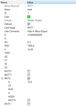
-
In the Model Browser, right-click and select .
A default PSHELL property displays in the Entity Editor.
- For Name, enter solid.
- For Material, click .
-
In the Select Material dialog, select
steel and click OK.
Figure 3. Assign the Material steel to the Property solid 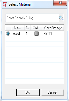
-
For Card Image, select PSOLID from the drop-down menu
and click Yes to confirm.
The property of the solid steel pipe has been created as 3D PSOLID. Material information is linked to this property.
Link Material and Property to Existing Structure
-
In the Model Browser, click on the
pipe component.
The component template displays in the Entity Editor.
- For Property, click .
-
In the Select Property dialog, select
solid and click
OK.
Figure 4. Assign the Property solid to the Component pipe 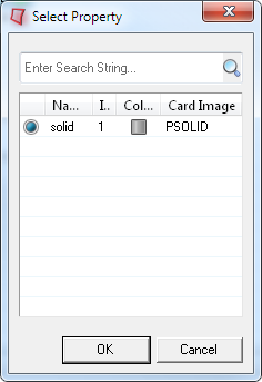
Apply Thermal Loads and Boundary Conditions to the Model
A structural constraint spc_struct is applied on the RBE2 element to fix the pipe on the ground. Two empty load collectors, spc_heat and heat_flux have been pre-created. In this section, the thermal boundary conditions and heat flux are applied on the model and saved in spc_heat and heat_flux, respectively.
Create Thermal Constraints
-
Click the Set Current Load Collector panel located at
the right corner of the footer bar, as shown below.
A list of load collectors appears.
Figure 5. Setting the Current Load Collector 
- Select spc_heat as the current load collector.
- From the Analysis page, click constraints.
- Go to the create subpanel.
- Click the entity selection switch and select nodes from the pop-up menu.
- Click .
-
Select the predefined entity set heat and click
select.
The selected nodes on the fixed end should be highlighted.
- Uncheck the boxes in front of dof1, dof2, dof3, dof4, dof5, and dof6 and enter 0.0 in the entry fields.
- Click load types = and select SPC from the pop-up list.
-
Click create.
This applies these thermal constraints to the selected nodal set.
- Click return to go to the Analysis page.
Create CHBDYE Surface Elements
- Click .
- For Name, enter heat_surf.
- For Card Image, select CONDUCTION from the drop-down menu.
- Select an appropriate color from the palette.
-
For Secondary Entity IDs, click Elements.
The Secondary Entity IDs panel is now displayed below the Graphics Browser.
- Click the switch button for elems and select faces from the pop-up list.
- Click the highlighted solid elems and select by sets from the pop-up selection menu.
- Select element set solid elems and click select.
- Click nodes in the face nodes field.
-
Select four nodes on one face of a solid element where the heat flux is
applied, as shown in Figure 1.
Figure 6. Nodes on the Surface Element 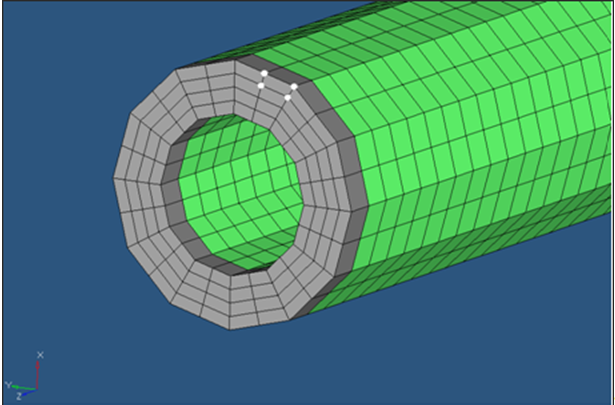
-
Click add.
This adds the CHBDYE surface elements on all the solid elements following the same side convention, as shown in Figure 2.
Figure 7. CHBDYE Surface Elements 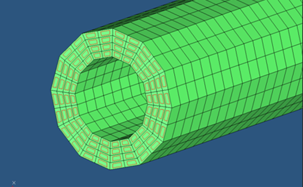
- Click return to return to the Entity Editor.
- Click Close.
Create Heat Flux on Surface Elements
- Set your current load collector to heat_flux.
- From the Analysis page, click flux to enter the Flux panel.
- Go to the create subpanel.
- Click .
-
Select heat_surf and click
select.
The surface elements are highlighted.
- Click load types= and select QBDY1.
- In the value= field, enter 1.0.
-
Click create.
The uniform heat flux in the surface elements is defined.
- Click return to go back to Analysis page.
Create Heat Transfer Load Step
-
In the Model Browser, right-click and select .
A default load step displays in the Entity Editor.
- For Name, enter heat_transfer.
- Click the drop-down menu in the Value field next to Analysis type in the Entity Editor and select Heat transfer (steady-state).
- For SPC, click .
-
In the Select Loadcol dialog, select
spc_heat and click OK.
Figure 8. Select the Constraints 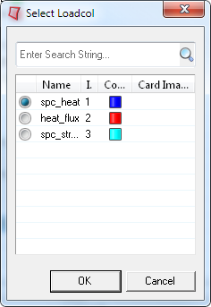
- For LOAD, click .
- In the Select Loadcol dialog, select heat_flux and click OK.
- Verify that the Analysis type is set to HEAT.
- Check the box next to OUTPUT.
- Activate the options of FLUX and THERMAL on the sub-list.
-
Under each result selection, click the space next to FORMAT and select
H3D format from the drop-down menu. For THERMAL,
click the Table icon
 and select
H3D from the drop-down menu in the table that
opens.
and select
H3D from the drop-down menu in the table that
opens.
-
Click the button under OPTION and select ALL, as shown
in Figure 2.
Flux and Thermal output can also be requested in the Control Cards panel on the Analysis page.
Figure 9. Setting up the Heat Transfer Loadstep 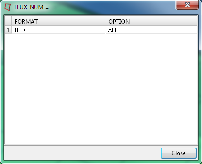
Create a Structure Load Step
-
In the Model Browser, right-click and
select .
A default load step displays in the Entity Editor.
- For Name, enter structure_temp.
- Click on the drop-down menu in the Value field next to Analysis type in the Entity Editor and select Linear Static.
-
For SPC, click Unspecified >
 .
.
- In the Advanced Selection dialog, select spc_struct and click OK.
- Select the check box next to TEMP_LOAD and SUBCASE OPTIONS.
- For SID, select SUBCASEID.
-
Click and select the heat transfer
subcase.
-
Click Apply.
This selects the heat transfer subcase ID as the input load for TEMP entry for the structural subcase.
Figure 10. Select Heat Transfer Subcase as Load for Structural Subcase 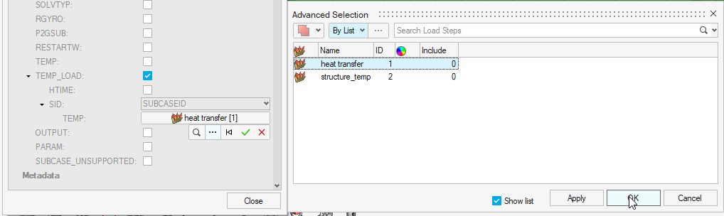
- Click Close.
Submit the Job
-
From the Analysis page, click the OptiStruct
panel.
Figure 11. Accessing the OptiStruct Panel 
- Click save as.
-
In the Save As dialog, specify location to write the
OptiStruct model file and enter
pipe_complete for filename.
For OptiStruct input decks, .fem is the recommended extension.
-
Click Save.
The input file field displays the filename and location specified in the Save As dialog.
- Set the export options toggle to all.
- Set the run options toggle to analysis.
- Set the memory options toggle to memory default.
- Click OptiStruct to launch the OptiStruct job.
View the Results
Gradient temperatures and flux contour results for the steady-state heat conduction analysis and the stress and displacement results for the structural analysis are computed from OptiStruct. HyperView is used to post-process the results.
View Heat Transfer Analysis Results
-
From the OptiStruct panel, click HyperView.
HyperView is launched and the results are loaded. A message window appears to inform of the successful model and result files loading into HyperView.
- Click Close to close the message window, if one appears.
-
On the Results toolbar, click
 to open the
Contour panel.
to open the
Contour panel.
-
Select Subcase 1 - heat transfer as the current load
case in the Results tab, as shown below.
Figure 12. Results tab in HyperView 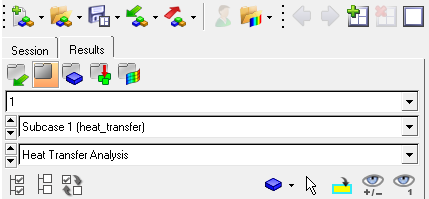
- In the Contour panel, select the first pull-down menu below Result type and select Element Fluxes (V).
-
Click Apply.
A contoured image representing thermal fluxes should be visible.
- Select the first pull-down menu below Result type and select Grid Temperatures (s).
-
Click Apply.
Both flux and temperature results are shown below.
Figure 13. Results of Heat Transfer Analysis 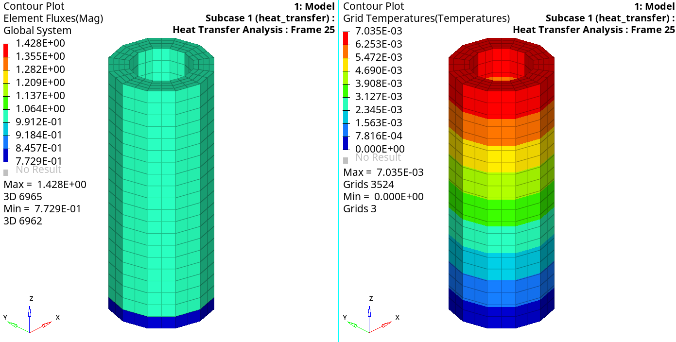
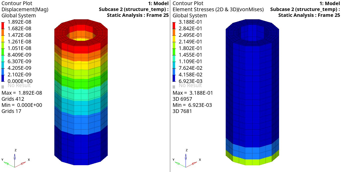
View the Results for the Coupled Thermal/Structure Analysis
- Select the structure analysis subcase as the current load case in the Load Case and Simulation Selection window.
- Select the first pull-down menu below Result type and select Element Stresses [2D & 3D] (t).
- Select the second pull-down menu below Result type and select vonMises.
-
Click Apply.
A contoured image representing von Mises stresses should be visible. Each element in the model is assigned a legend color, indicating the von Mises stress value for that element, resulting from the applied loads and boundary conditions.
- Select the first pull-down menu below Result type and select Displacement (v).
- Select the second pull-down menu below Result type and select Mag.
-
Click Apply.
Both stress and displacement contours are shown below.
Figure 14. Results of the structural analysis