OS-T: 1085 Linear Steady-state Heat Convection Analysis
This tutorial performs a heat transfer analysis on a steel pipe.

Launch HyperMesh and Set the OptiStruct User Profile
-
Launch HyperMesh.
The User Profile dialog opens.
-
Select OptiStruct and click
OK.
This loads the user profile. It includes the appropriate template, macro menu, and import reader, paring down the functionality of HyperMesh to what is relevant for generating models for OptiStruct.
Import the Model
-
Click .
An Import tab is added to your tab menu.
- For the File type, select OptiStruct.
-
Select the Files icon
 .
A Select OptiStruct file browser opens.
.
A Select OptiStruct file browser opens. - Select the thermal.fem file you saved to your working directory.
- Click Open.
- Click Import, then click Close to close the Import tab.
Set Up the Model
Create Thermal Material and Properties
-
In the Model Browser, right-click and select .
A default MAT1 material displays in the Entity Editor.
- For Name, enter steel.
-
Check the box in front of MAT4.
MAT4 card image appears below MAT1 in the Entity Editor. The MAT1 card defines the isotropic structural material. MAT4 card is for the constant thermal material. MAT4 uses the same material ID as MAT1.
-
Enter the following values for the material, steel, in the Entity Editor.
- [E] Young's modulus
- 2.1 x 10¹¹ Pa
- [NU] Poisson's ratio
- 0.3
- [RHO] Material density
- 7.9 x 10³ Kg/m3
- [A] Thermal expansion coefficient
- 1.0 x 10⁻⁵ / °C
- [K] Thermal conductivity
- 73W / m °C
- [H] Heat transfer coefficient
- 40W / m2 °C
Figure 2. Material Entity Editor 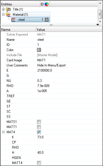
A new material, steel, is created with both structural and thermal properties.
-
In the Model Browser, right-click and select .
A default PSHELL property displays in the Entity Editor.
- For Name, enter solid.
- For Card Image, select PSOLID and click Yes to confirm.
- For Material, click .
-
In the Select Material dialog, select
steel and click OK.
The property of the solid steel pipe has been created as 3D PSOLID. Material information is linked to this property.
Link Material and Property to Existing Structure
-
In the Model Browser, click the component
pipe.
The Entity Editor opens.
- For Property, click .
-
In the Select Property dialog, select
solid and click OK.
The material steel now is automatically linked to the component pipe.
Apply Thermal Loads and Boundary Conditions
In this exercise the thermal boundary conditions are applied on the model and saved in a predefined load collector spc_temp. A predefined node 4679 specifies the ambient temperature. A predefined node set node_temp contains the nodes on the inside surface of the pipe.
Create Temperature on the Inner Surface of the Pipe
- From the Analysis page, click constraints.
- Go to the create subpanel.
- Make sure the current selection field is set to nodes.
- Click .
- Select node_temp and click select.
- Uncheck the box in front of dof1, dof2, dof3, dof4, dof5, and dof6 and verify that the entry fields are set to 0.0.
- Set load types = to SPC.
-
Click create.
This applies the temperature 0.0 on the inside nodes. In the next step, the temperature value is updated to 60.
-
Click the Card edit icon
 .
.
- Click .
- Check the box in front of spc_temp and click select.
- Click config= and select const.
- Click type= and select SPC.
- Click edit.
- In the field of D, enter 60.0.
- Click return three times to go back to the Analysis page.
Create Ambient Temperature
- From the Analysis page, select the Constraints panel.
- Go to the create subpanel.
- Click .
-
Input the ID of the predefined node
4679.
Node 4679 should be highlighted.
- Uncheck the box in front of dof1, dof2, dof3, dof4, dof5, and dof6 and verify that the entry fields are set to 0.0.
- Click create.
-
Click the Card edit icon .
- Select loads entry.
- Select the ambient spc just created on the screen.
- Click config= and select const.
- Click type= and select SPC.
- Click edit.
-
In the field of D, enter 20.0.
The temperature boundary conditions are created, as shown below.
Figure 3. Thermal Boundary Conditions 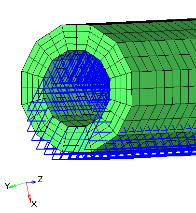
- Click return three times to go back to the Analysis page.
Create CHBDYE Surface Elements
- Click .
- For Name, enter convection.
- For Card Image, select CONVECTION from the drop-down menu.
- Click Color and select a color from the palette.
- Click MID to activate it.
- For Material, click .
-
In the Select Material dialog, select steel and click
OK.
An element group convection and a free convection property PCONV are created.
-
For Secondary Entity IDs, select Elements.
A panel appears under the modeling window.
- Click on the switch button beside elems and select faces from the list.
- Click the highlighted solid elems and select by sets from the selection menu.
- Select element set elem_convec and click select.
- Click nodes in face nodes field.
-
Select 4 nodes on the surface face of a solid element, as shown below.
Figure 4. Selected Surface Nodes on the Solid Element Outside the Pipe 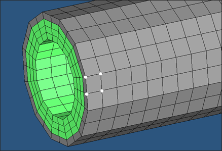
- In the break angle = field, enter 89.0.
-
Click add.
This adds the CHBDYE surface elements to the solid elements on the outer surface following the same side convention, as shown below.
Figure 5. Surface Elements on the Outer Layer of the Pipe 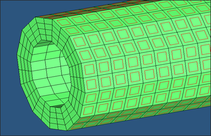
- Click return to go back to the Create group window.
Define Convection Boundary Condition to Surface Elements
-
Click the Card Edit icon .
- Select elems.
- Click elems > by group.
- Check the box in front of CONVECTION and click select.
- Click config= and select second4.
- Click type= and select CHBDYE4.
- Click edit and go to the CHBDYE Card Image panel.
- Check the box in front of CONV.
-
Click TA1 and input the ambient node ID
4679, as shown below.
Figure 6. Define the Convection Boundary Condition 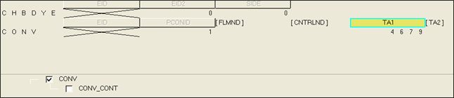
- Click return three times to go back to the Analysis page.
Create Heat Transfer Load Step
- In the Model Browser, right-click and select .
- A default loadstep displays in the Entity Editor.
- For Name, enter heat_transfer.
- Click on the Analysis type field and select Heat transfer (steady-state) from the drop-down menu.
- For SPC, click .
- In the Select Loadcol dialog, select spc_temp and click OK.
- Check the box next to Output.
- Activate the options of FLUX and THERMAL on the sub-list.
- Activate the FORMAT fields for both outputs and select H3D format.
-
Activate the OPTION fields for both outputs and select
ALL.
The FORMAT and OUTPUT fields for THERMAL output may open up a new window. Click on the first field in the window to select the corresponding values.
FLUX and THERMAL output can also be requested in the Control cards panel on the Analysis page.
Submit the Job
-
From the Analysis page, click the OptiStruct
panel.
Figure 7. Accessing the OptiStruct Panel 
- Click save as.
-
In the Save As dialog, specify location to write the
OptiStruct model file and enter
thermal_complete for filename.
For OptiStruct input decks, .fem is the recommended extension.
-
Click Save.
The input file field displays the filename and location specified in the Save As dialog.
- Set the export options toggle to all.
- Set the run options toggle to analysis.
- Set the memory options toggle to memory default.
- Click OptiStruct to launch the OptiStruct job.
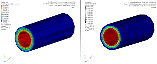
View the Results
Gradient temperatures and flux contour results for the steady-state heat conduction analysis and the stress and displacement results for the structural analysis are computed from OptiStruct. HyperView will be used to post process the results.
-
From the OptiStruct panel, click HyperView.
HyperView is launched and the results are loaded. A message window appears to inform of the successful model and result files loading into HyperView.
- Click Close to close the message window, if one appears.
-
On the Results toolbar, click
 to open the
Contour panel.
to open the
Contour panel.
- Select the first pull-down menu below Result type and select Grid Temperatures(s).
-
Click Apply.
You may have to use Edit Legend in the Contour panel to get the contour, as shown in Figure 8.A contour plot of grid temperatures is created.
- Select the first pull-down menu below Result type and select Element Fluxes (V).
-
Click Apply.
You may have to use Edit Legend in the Contour panel to get the contour. Both temperature and flux contour plots are shown in Figure 8.
Figure 8. Results of Heat Transfer Analysis