OS-T: 1060 Analysis of a Composite Aircraft Structure using PCOMPG

This tutorial takes you through the process of developing a ply lay-up definition for a composite structure using a PCOMPG card, and shows the advantages of post-processing the results with global ply numbers. The traditional definition method, using PCOMP, is introduced first here to ultimately show the practical advantages of using PCOMPG for the given scenario.

Before you begin, copy the file(s) used in this tutorial to your working directory.

frame.hm

Figure 1 illustrates the model for this tutorial. Since the structure, loads, and boundary conditions are symmetrical about the x-axis, only one half of the structure is modeled with suitable boundary conditions applied to enforce half symmetry.

Launch HyperMesh and Set the OptiStruct User Profile

Launch HyperMesh.
The User Profile dialog opens.
Select OptiStruct and click OK.
This loads the user profile. It includes the appropriate template, macro menu, and import reader, paring down the functionality of HyperMesh to what is relevant for generating models for OptiStruct.

Open the Model

Click File > Open > Model.
Select the frame.hm file you saved to your working directory.
Click Open.
The frame.hm database is loaded into the current HyperMesh session, replacing any existing data.

Review the Model Setup

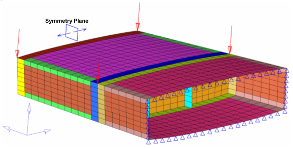
The structural model has been already set up and can be solved without any further modifications. Review the model setup before submitting the job.

The model is set up for Linear Static Analysis. As mentioned earlier, only half of the structure is modeled; and to impose the half symmetry boundary conditions, all the nodes on the symmetry plane are constrained in DOF1, DOF5, and DOF6.

All of the components are modeled with the PCOMP property which lists the plies (stacking sequence) from the bottom surface upwards, with respect to the element's normal direction, as shown in Figure 2.

Figure 2. Ply Stacking Sequence with Respect to Element Normal

Components in this model that have names starting with the word "Flange" represent junctions in which different components are connected together. While reviewing, closely watch the flange area formed by the Skin and Rib components (highlighted in the following figure). Review the ply lay-up of the Skin_inner, Rib, Flange1_Rib_Skin, and Flange2_Rib_Skin components (laminate layout is shown in the bottom portion of the following figure).

Note: Few plies are common for the Skin_inner, Flange1_Rib_Skin, Flange2_Rib_Skin, and Skin_outer components, but appear in different stacking sequence in each component. For example, the 4th ply in Skin_inner is the 3rd ply in Flange2_Rib_Skin and the 2nd ply in the Skin_outer components.

ply_stack_2 — Figure 3. Ply stacking for the Skin_inner, Rib, Skin_outer, Flange1_Rib_Skin, and Flange2_Rib_Skin Components

From the 2D page, click HyperLaminate.
This opens the HyperLaminate GUI, in which the ply lay-up information can be defined, reviewed and edited. Material properties and design variables can also be created and edited here.
Expand the Laminates portion of the tree structure on the left-hand side of the screen.
Select the Skin_inner PCOMP.
Details of the laminate appear in the GUI.
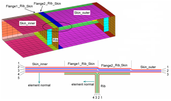
Verify that the lay-up definition for Skin_inner matches the first 5 entries of the table below, which is the lay-up information of Flange1_Rib_Skin component.
Select the Rib PCOMP and verify that the 3rd and 4th lay-up definition for Rib matches the 6th and 7th entries in the following table.

Select the Flange1_Rib_Skin PCOMP to view the ply lay-up definitions. Verify that the lay-up definition for Flange1_Rib_Skin matches the following table.

Notice that the first 5 layers are the same as Skin_inner lay-ups and that the last two lay-ups are the same as the 3rd and 4th lay-up of Rib, as shown in the last figure. You can verify how other flanges are modeled.

Table 1. Laminate properties of Flange1_Rib_Skin
Ply Number	Material	Thickness T	Orientation	SOUT
1	carbon_fiber	1.2	45	YES
2	matrix	0.2	90	YES
3	carbon_fiber	1.2	-45	YES
4	matrix	0.2	-90	YES
5	carbon_fiber	1.2	90	YES
6	matrix	0.2	-45	YES
7	carbon_fiber	1.2	45	YES

You can also review the other components. Once the review is completed, select File > Exit to exit the HyperLaminate GUI and return to HyperMesh.

Submit the Job

From the Analysis page, click the OptiStruct panel.

Figure 4. Accessing the OptiStruct Panel
Click save as.
In the Save As dialog, specify location to write the OptiStruct model file and enter frame_PCOMP for filename.
For OptiStruct input decks, .fem is the recommended extension.
Click Save.
The input file field displays the filename and location specified in the Save As dialog.
Set the export options toggle to all.
Set the run options toggle to analysis.
Set the memory options toggle to memory default.
Click OptiStruct to launch the OptiStruct job.

If the job is successful, new results files should be in the directory where the frame_PCOMP.fem was written. The frame_PCOMP.out file is a good place to look for error messages that could help debug the input deck if any errors are present.

The default files written to the directory are:

frame_PCOMP.html: HTML report of the analysis, providing a summary of the problem formulation and the analysis results.
frame_PCOMP.out: OptiStruct output file containing specific information on the file setup, the setup of your optimization problem, estimates for the amount of RAM and disk space required for the run, information for each of the optimization iterations, and compute time information. Review this file for warnings and errors.
frame_PCOMP.h3d: HyperView binary results file.
frame_PCOMP.res: HyperMesh binary results file.
frame_PCOMP.stat: Summary, providing CPU information for each step during analysis process.

View the Results/Post-processing

Click HyperView from the OptiStruct panel.
HyperView launches and the model results are automatically loaded.
Click Close to close the message window.
Click the Contour toolbar .
Select the first switch below Result type and select Composite Stresses(s).
Select the second switch and select the P1 (major) Stress.
Select 3 for the Layers option.
In the field below Averaging method, select None.

Figure 5.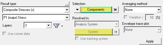
Click Apply.
This contours the maximum principle stress for the 3rd ply of all the components in the model.
Click the Isometric View icon in the Standard Views toolbar to see the model, as shown in the following figure.

Figure 6. Stress Distribution on the Top Face of the Frame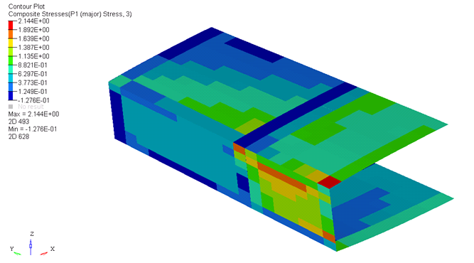

The stress value does not vary gradually in the top face region, but suddenly decreases to a lower value across the Flange2_Rib_Skin component.

Looking at the table of laminate properties of Flange1_Rib_Skin again, observe that the 3rd ply property of the Flange2_Rib_Skin component is of a matrix material and the third plies in the components adjacent to it (Flange1_Rib_Skin and Skin_outer) are of a carbon fiber material. The sudden changes in the stress values occur because stress on two different materials is being shown. This example shows that, for the results to be meaningful during post-processing of the PCOMP results, you have to correlate the ply results to their corresponding ply property.

This highlights that during the post-processing of PCOMP components, plotting results based on only the ply number is not sufficient. The ply properties (material, thickness, orientation, failure index, etc.) must be kept track of during post-processing with this method. In cases that use large and complex models, it becomes tedious to track the individual ply properties during post-processing.

This drawback to using PCOMP can be avoided with the use of the PCOMPG card for property definition. Using the PCOMPG card, you can assign a global ply number for each ply and post-process the results based on global ply number. The following steps explain the procedure to redefine the model with PCOMPG property.

Redefine the Model Setup

Close the HyperView window and return to HyperMesh.

Tip: Click to return to the previous page where HyperMesh is open, if you are using HyperMesh Desktop.
From the 2D page, select the HyperLaminate panel.
This opens the HyperLaminate GUI in which the ply lay-up information can be defined, reviewed and edited.
Click Tools > Laminate Options.
This opens a new window in which the default ply lay-up options can be set.
Click the Convention switch and select Total.
Click OK to close the window.
This sets up Total as the default option whenever a new component is created.
Figure 7. Laminate Information with Global Ply Number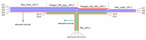

Now you create new PCOMPG components with global ply numbers defined as shown in Figure 7. As discussed earlier, the 4th ply in Skin_inner is the 3rd ply in Flange2_Rib_Skin and the 2nd ply in Skin_outer components. Therefore, all of these plies will be defined with the same global ply ID 4. Similarly, all other plies are to be defined, as shown in Figure 7.

Expand the laminates portion of the tree structure on the left-hand side of the screen.
Right-click PCOMPG.
A menu appears.
Click New.
This creates new component, which is named NewLaminate1 by default, and the tree structure is expanded.
Rename the component to Skin_inner_GPLY by right-clicking and select Rename in the text field and overwrite the default component name.
In the Add/Update plies section, under the field GPLYID, enter 1.
Select the pull-down menu below Material and select carbon_fiber.
Below the Thickness T1 field, enter 1.2.
Below the Orientation field, enter 45.
Select the pull-down menu below SOUT and select YES.
Click Add New Ply to add the ply information.

Repeat this procedure to add 4 more plies with the properties shown in the table:


GPLYID	Material	Thickness T	Orientation	SOUT
2	matrix	0.2	90	YES
3	carbon_fiber	1.2	-45	YES
4	matrix	0.2	-90	YES
5	carbon_fiber	1.2	90	YES

Click Update Laminate at the bottom of the window to update the lay-up information.
The graphical display of lay-up information now appears in the field below the Review tab, on the right side of the GUI.

Create a new PCOMPG component with name Rib_GPLY and the ply lay-up, as shown in the following table:


GPLYID	Material	Thickness T	Orientation	SOUT
11	carbon_fiber	1.2	0	YES
12	matrix	0.2	45	YES
13	matrix	0.2	-45	YES
14	carbon_fiber	1.2	45	YES

Refer to Figure 7 to create the Flange1_Rib_Skin_GPLY component.

Right-click Skin_inner_GPLY and select Duplicate from the menu to create an identical component.
Rename the component as Flange1_Rib_Skin_GPLY by right-clicking and selecting rename.

Add 2 more plies with the properties shown in the following table using the Add New Ply feature.


GPLYID	Material	Thickness T	Orientation	SOUT
13	matrix	0.2	-45	YES
14	carbon_fiber	1.2	45	YES

The new component Flange1_Rib_Skin_GPLY was created. Its first 5 plies are the same as Skin_inner_GPLY and its last 2 plies are the 3rd and 4th plies of the Rib component.

To reduce the number of steps in this tutorial, the ply lay-up information of other components is already defined with PCOMPG property and appropriate laminate information in the updated_PCOMPG_properties.fem file you saved to your working directory. This file is imported into HyperMeshto update (overwrite) the properties instead of manually updating them.

The updated_PCOMPG_properties.fem file is saved in OptiStruct input file format. Open this in any text editor to review how the components are defined with PCOMPG properties. A section of the file is shown below.

comps_def — Figure 8. Components defined with PCOMPG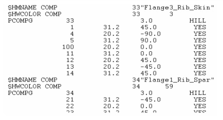

Click File > Exit to exit the HyperLaminate GUI and return to HyperMesh.
Click File > Import > Solver Deck.
Click the toggle to expand the Import options and check the box next to FE overwrite.
This option overwrites the old PCOMP properties with PCOMPG properties defined in the updated_PCOMPG_properties.fem file.
Click on the folder icon next to File, select the updated_PCOMPG_properties.fem file and click Import.
Click Close.

Review the Imported Properties in HyperLaminate

From the 2D page, go to the HyperLaminate panel.
Expand the laminates portion of the tree structure on the left-hand side of the screen.
All of the components now appear under PCOMPG. The components created earlier (Skin_inner_GPLY, Rib_GPLY, and Flange1_Rib_Skin_GPLY) are still present. There is no element associated with these components. Review the PCOMPG components to view the laminate definitions.
Click File > Exit.

Submit the Job

From the Analysis page, click the OptiStruct panel.

Figure 9. Accessing the OptiStruct Panel
Click save as.
In the Save As dialog, specify location to write the OptiStruct model file and enter frame_PCOMPG for filename.
For OptiStruct input decks, .fem is the recommended extension.
Click Save.
The input file field displays the filename and location specified in the Save As dialog.
Set the export options toggle to all.
Set the run options toggle to analysis.
Set the memory options toggle to memory default.
Click OptiStruct to launch the OptiStruct job.

If the job is successful, new results files should be in the directory where the frame_PCOMPG.fem was written. The frame_PCOMPG.out file is a good place to look for error messages that could help debug the input deck if any errors are present.

The default files written to the directory are:

frame_PCOMPG.html: HTML report of the analysis, providing a summary of the problem formulation and the analysis results.
frame_PCOMPG.out: OptiStruct output file containing specific information on the file setup, the setup of your optimization problem, estimates for the amount of RAM and disk space required for the run, information for each of the optimization iterations, and compute time information. Review this file for warnings and errors.
frame_PCOMPG.h3d: HyperView binary results file.
frame_PCOMPG.res: HyperMesh binary results file.
frame_PCOMPG.stat: Summary, providing CPU information for each step during analysis process.

View the Results/Post-processing

From the OptiStruct panel, click HyperView.
HyperView is launched and the results are loaded. A message window appears to inform of the successful model and result files loading into HyperView.
Click Close to close the message window, if one appears.
On the Results toolbar, click to open the Contour panel.
Select the first switch below Result type and select Composite Stresses (s).
Select the second switch and select P1 (major) Stress.
For the Layers field, select PLY 3.
For Averaging method, select None.
Click Apply.
This plots the maximum principle stress for global ply 3. The results are not plotted in the regions where global ply 3 is not present.
Click the Isometric View icon in the Standard Views toolbar.

Figure 10.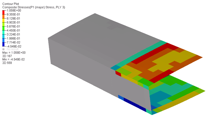

Post-processing the results based on global ply number eliminates the need to track the ply number and corresponding ply properties on the components. The results are displayed based on the global ply number, irrespective of the ply order, so you can chose any one global ply number and view results across the whole component. If a particular ply is not present in any given region, no result is displayed.