
OS-T: 1050 Connection of Dissimilar Meshes using CWELD Elements
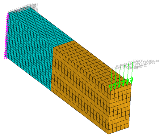
In this tutorial, an existing finite element model of a simple cantilever beam is used to demonstrate how to connect dissimilar meshes using CWELD elements.
Before you begin, copy the file(s) used in this tutorial to your
working directory.
Launch HyperMesh and Set the OptiStruct User Profile
-
Launch HyperMesh.
The User Profile dialog opens.
-
Select OptiStruct and click
OK.
This loads the user profile. It includes the appropriate template, macro menu, and import reader, paring down the functionality of HyperMesh to what is relevant for generating models for OptiStruct.
Open the Model
- Click .
- Select the dissimilar.hm file you saved to your working directory.
-
Click Open.
The dissimilar.hm database is loaded into the current HyperMesh session, replacing any existing data.
Set Up the Model
Create CWELD Elements
-
In the Model Browser, right-click and select .
A default PSHELL property template displays in the Entity Editor.
- For Name, enter welds.
- For Card Image, select PWELD from the drop-down menu and click Yes to confirm.
- For Material, click .
- In the Select Material dialog, select steel and click OK.
-
For D (weld diameter), enter 0.1.
This creates a new property definition named welds.
- In the Model Browser, right-click and select .
- For Name, enter welds.
-
Click Color and select a color.
This creates the new component named welds.
- From the 1D page, click spotweld.
- Make sure the using elems subpanel is selected.
- Click .
- Click the switch under element config and select rod from the pop-up menu.
- Click property = and select welds from the list of properties.
- Click search tolerance = and enter 0.1.
- Click and select the membrane_fine collector.
-
Click create.
A weld element is created at each node on the fine-mesh matching face. A number of plot elements are created too, these are helpful to find the elements attached when looking for the welds.
- Click return to go back to the main menu.
Submit the Job
-
From the Analysis page, click the OptiStruct
panel.
Figure 2. Accessing the OptiStruct Panel 
- Click save as.
-
In the Save As dialog, specify location to write the
OptiStruct model file and enter
dissimilar for filename.
For OptiStruct input decks, .fem is the recommended extension.
-
Click Save.
The input file field displays the filename and location specified in the Save As dialog.
- Set the export options toggle to all.
- Set the run options toggle to analysis.
- Set the memory options toggle to memory default.
- Click OptiStruct to launch the OptiStruct job.
The default files written to the directory are:
- dissimilar.html
- HTML report of the analysis, providing a summary of the problem formulation and the analysis results.
- dissimilar.out
- OptiStruct output file containing specific information on the file setup, the setup of your optimization problem, estimates for the amount of RAM and disk space required for the run, information for each of the optimization iterations, and compute time information. Review this file for warnings and errors.
- dissimilar.h3d
- HyperView binary results file.
- dissimilar.res
- HyperMesh binary results file.
- dissimilar.stat
- Summary, providing CPU information for each step during analysis process.
Post-process the Results
View Displacement Contour
-
From the OptiStruct panel, click HyperView.
HyperView is launched and the results are loaded. A message window appears to inform of the successful model and result files loading into HyperView.
-
Set the animation type to Linear
 .
.
-
On the Results toolbar, click
 to open the
Contour panel.
to open the
Contour panel.
- Select the first pull-down menu below Result type: and select Displacement (v).
-
Click Apply.
The resulting colors represent the displacement field resulting from the applied loads and boundary conditions.
-
Click the Page Layout icon
 on the toolbar.
-
Choose the second layout in the first row of the pop-up window.
This changes the modeling window in two separate windows. The left window will have the previously loaded model and the right window will be blank.
- Load the control example in the right side window to compare the results.
-
Click the right-hand pane in the display area.
A blue line appears around the window to show that it is selected.
-
Click the Load Result icon
 in the toolbar.
-
Click Load Model
 and select the file control.h3d
you saved to your working directory as both the model and results file.
and select the file control.h3d
you saved to your working directory as both the model and results file.
- Click Apply.
-
Right-click on the left pane and activate menu .
This option applies results from the current window to the new window. You can now visually compare the displacement results from the dissimilar mesh model with a uniform mesh model.
View the Results
- Select the left-hand panel in the display area.
-
On the Results toolbar, click to open the
Contour panel.
- Under Result type, select Element Stresses (2D & 3D)(t) and vonMises.
- In the field below Averaging method, select None.
- Click Apply.
-
Right-click on the left pane and activate menu .
You can now visually compare the von Mises stress results from the dissimilar model with a uniform mesh model.