
Perform General Signal Processing for Computational Aeroacoustics
Process a surface or volume output or point probe file created from data as a part of the General Signal Processing (GSP) workflow that is utilized for Computational Aeroacoustics (CAA).
Examples of this workflow include the post-processing of a rotating fan and interior noise propagation simulations. You may process time-dependent point, surface or volume data to interpret the noise source from aerodynamic and aeroacoustic simulations.
Hydrodynamic Contour Map Creation
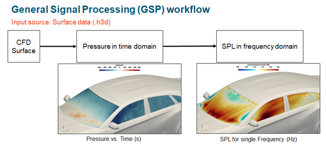
The purpose of the GSP workflow is to generate hydrodynamic surface/volume contour maps from a time-dependent surface/volume output containing pressure or velocity, written in HyperView (.h3d) format.
The source .h3d file must be created directly from the solver (merged .h3d) or converted from merged ENSIGHT data (.case files) via the HVTrans application. The source file should contain the time-dependent pressure for one or more surfaces at a high enough frequency and long enough duration to support the requested frequency range of interest.
Using the source time-dependent pressure map, you can obtain the Sound Pressure Level (SPL) in decibels (dB) or weighted levels to represent human hearing more closely in dB(A) or dB(C). When the source data contains time-dependent velocity, you can obtain the Power Spectrum in Pa2. The SPL or power spectrum can be obtained for a single range of frequencies [fmin, fmax] represented at the center of the broadband, or optionally, integrated for each fractional octave band across the requested frequency spectrum. The SPL is obtained by computing the Fast Fourier Transform (FFT) of the time dependent pressure signal, modifying the resultant power spectral density and logarithmically rescaling, accounting for the reference pressure of air for each element present on the surface of interest. The value for SPL is computing by using the relationship shown in Equation 1. Figure 1 provides an example of the data that is utilized and created during the GSP workflow.
The above equation represents the sound pressure level of ith element on a given surface, using Pref=2.0e-5Pa. Where SPL has units of decibels (dB). When required, the power spectrum of velocity can be obtained by selecting the appropriate input variable (velocity component or velocity magnitude) and processing the data as explained for SPL.
-
From the Post ribbon, click the .
Figure 2. 
-
Define the surface- or volume-based signal processing attributes in the
dialog.
Figure 3. Input dialog for GSP (Hydrodynamic Contour Map focus) 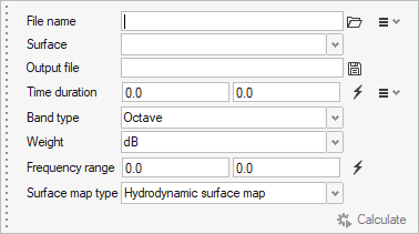
-
Load the data file of interest into the tool using the file browser icon,
 .
Fields are populated with the data that is contained in the input source (.h3d).
.
Fields are populated with the data that is contained in the input source (.h3d). -
The following attributes are populated once the data is initially loaded.
Assign each of the attributes according to best-practice guidelines.
- File name
- Source data as provided from the solver (.h3d file) or the pre-processed compact form of the pressure/velocity vs. time signal (.gsph5 file).
- Surfaces/Volumes
- Surface or volume components that are sent to the GSP algorithm. Multiple components contained within the input source may be selected by entering the advanced selection context.
- Variables
- Input variables that define the input signal. Multiple variables may be selected and processed at the same time.
- Time duration
- Beginning and ending time values in seconds. The fields may be
modified based to control the number of records considered during
the calculation. Auto-calculate
 can be utilized to redefine the
original time-series bounds.
can be utilized to redefine the
original time-series bounds. - Band type
- Output band summation option. Single band provides a single dB map comprised of SPL from the full frequency range. Octave (fractional octave) provides a frequency dependent dB map for each of the Nth octave bands, with N=1, 3, 12 that fall within the frequency range of interest. The octave band center frequency is reported within the output file.
- Weight (Scaling)
- Decibel scaling for dB (default), dBA or dBC. All data in the dB map
will be weighted according to your selection of weight. Provides dBA
weight for interpreting dB maps associated with the range of human
hearing.Note: dBA ~= dB at a frequency of 1kHz.
- Frequency range
- Minimum and maximum cutoff frequency to be displayed in the output
results. Auto-calculate can be utilized to redefine the
original supported cutoff frequency bounds.Note: The minimum value is set to resolve the minimum frequency that is supported by ~4 cycles of the transient period, the maximum is set to the Nyquist Frequency.
-
Define any additional options that are needed to compute the hydrodynamic
contour map and band filtered animation through the two additional menu icons in
the main menu dialog. Select the FFT parameters through the first menu, as shown
in Figure 4.
Figure 4. FFT parameters for the GSP calculation 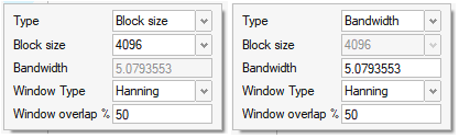
- Type
- Modifies the subsequent selection of the FFT bandwidth for
windowing.
When Type=Block size, the Block size enumerated list is accessible, defaulting to 4096 records. The associated Bandwidth for that Block size is automatically calculated and presented to you.
When Type=Bandwidth size, the Bandwidth real number is accessible, defaulting to the bandwidth associated with a Block size of 4096 records. When the Bandwidth is modified, the associated Block size is automatically calculated and presented to you.
- Window Type
- Windowing algorithm used to reduce spectral leakage that may be present within the input pressure signal. Hanning, Hamming and Blackman are available.
- Window Overlap (%)
- Define the percentage overlap for each window used during the FFT of the input pressure signal.
-
Review the data contained within the input source through the second
menu.
The menu shows the Time range (seconds), Record length (samples), Data Frequency (Hz) and Time step (seconds).
Figure 5. Source data parameters, non-modifiable 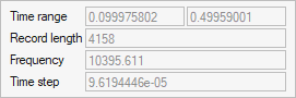
-
Once the parameters have been defined, click
Calculate.
- Retain input
- Setting the Retain input Boolean true will enable the application to
store the input data time-dependent / nodal-dependent signal to the
resulting output file. In this case, the original source data may be
deleted as it would no longer be needed.Note: When the Retain input option is selected, the output file will be significantly large, approximately equal to the source dataset when compressed.
- Compression level
- The output file may be compressed using HDF based file compression
according to your needs. High results in the highest level of
compression and smallest output file.Note: To reduce the output size as much as possible, you should not retain the input data and set the compression level to High.
This performs the calculation in a sub-process, allowing you to return to the UI and prepare any additional post-processing content. During the calculation, a status indicator is updated with the progress of the sub-process. To query the status of the calculation, press the
 icon.
icon.Once the calculation is complete, you are presented with the option to load the data into the post-processing session, as shown in Figure 6. Multiple datasets may be loaded into the session at once if required.
Note: Once the calculation has been completed, the definition for the GSP is stored in session, accessible in the Post Browser for future inspection.Figure 6. GSP progress bar and results complete, load data into the post-processing session 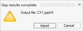
Figure 7. 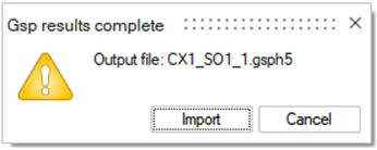
Band Filtered Transient Animation Summary
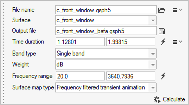
Provides a workflow to generate a Band Filtered Transient Surface Animation (BAFA) from a time-dependent source file, written in HyperView (.h3d) format.
Utilizing the same source input file as described in the hydrodynamic contour map summary, you can generate a BAFA according to the frequency range of interest. As in the hydrodynamic map process, the source file should contain the time-dependent pressure or pressure for one or more surfaces or volumes at a high enough frequency and long enough duration to support the requested frequency range of interest. If previously computed, or with the contour map type option: Both, the BAFA will utilize the FFT and filter the time domain data for output.
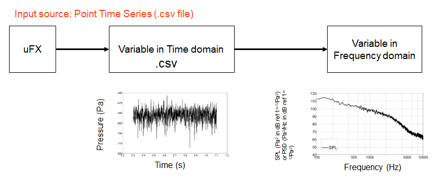
Point Probe Summary
Provides a workflow to compute noise levels from point probe measurement files using .csv files created directly from ultraFluidX.
-
From the Post ribbon, click the tool.
Figure 10. 
-
Define the point probe-based signal processing attributes in the dialog.
Figure 11. Input dialog for GSP (Point Probe focus) 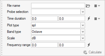
-
Load the data file of interest into the tool using the file browser icon,
.
Fields are populated with the data that is contained in the input source (.csv).
-
The following attributes are populated once the data is initially loaded
(Figure 12).
Assign each of the attributes according to best-practice guidelines.
- File name
- Source data as provided from the solver (.csv file).
- Probe selection
-
All, individual, or a subset of probes (read from the header names) for 1D processing. The advanced selection context may be used to chose specific probes.
- Time duration
- Beginning and ending time values in seconds. The fields may be
modified based to control the number of records considered during
the calculation. Auto-calculate can be utilized to redefine the
original time-series bounds.
- Plot type
- Define output plot type. Sound Pressure Level (SPL) or Power Spectral Density (PSD).
- Band type
- Output band summation option. Narrowband provides the full spectrum of requested frequency range output at the data source sampling frequency. Octave (fractional octave) provides a frequency dependent dB map for each of the Nth octave bands, with N=1, 3, 8, 12 that fall within the frequency range of interest. The octave band center frequency is reported for the computed bands.
- Weight
- Decibel weighting for dB (default), dBA or dBC. All data in the dB
map will be weighted according to your selection of weight. Provides
dBA weight for interpreting dB maps associated with the range of
human hearing.Note: dBA ~= dB at a frequency of 1kHz.
- Frequency range
- Minimum and maximum cutoff frequency to be displayed in the output
results. Auto-calculate can be utilized to redefine the
original supported cutoff frequency bounds.Note: The minimum value is set to resolve the minimum frequency that is supported by ~4 cycles of the transient period, the maximum is set to the Nyquist Frequency.
Figure 12. Populated input dialog for GSP (Point Probe focus) 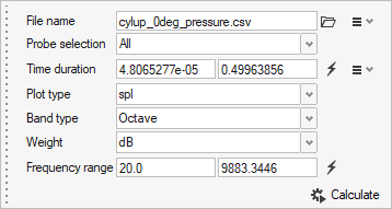
Batch Automation of GSP Surface Workflow
The GSP workflow can be utilized by running an automation script that generates the hydrodynamic contour map or BAFA without the user interacting with the GUI.
The batch automation can be accessed within the same distribution as the GUI (HWDesktop – HMCFD) from the command line. For example:
"<install_directory> \hwdesktop\hwx\plugins\hwd\profiles\HyperworksCfd\hwcfdGsp.bat" gspParams.json<install_directory>/altair/scripts/hmcfdgsp gspParams.jsonWhere the .json file contains the attributes that were provided in the GUI workflow, referenced above, and stored as follows (by default, in the application launch directory).
{
    "gspArgs": {
        "resultFilePath": "uFX_volumeData/Volume_Output_1_h3d/uFX_output.h3d",
        "outGspFname": "uFX_output_Power_Spectrum.gsph5",
        "partName": [
            "fluid_volume_default"
        ],
        "resultsName": "fluid_volume_default",
        "useCellData": true,
        "dataArrayName": [
            "velocity_magnitude"
        ],
        "timeRange": [
            0.62463957,
            0.8253299
        ],
        "bandType": "octave",
        "scale": "",
        "frequencyRange": [
            20.0,
            7623.6857
        ],
        "surfaceMapType": 0,
        "exportData": 0,
        "exportStride": 0,
        "exportDataFilename": "out",
        "exportResultType": 0,
        "compressionLevel": 0,
        "skipWritingTimeData": true,
        "skipWritingPsd": false,
        "logFile": "uFX_output_Power_Spectrum.log"
    },
    "fftArgs": {
        "nperseg": 512,
        "noverlap": 256,
        "window": "hann"
    }
}
{
    "gspArgs": {
        "resultFilePath": "CX1_SO1.h3d",
        "outGspFname": "BAFA_20-4000Hz.gsph5",
        "partName": [
            "c_front_window"
        ],
        "resultsName": "c_front_window",
        "useCellData": true,
        "dataArrayName": [
            "pressure"
        ],
        "timeRange": [
            1.12801,
            1.99815
        ],
        "bandType": "octave",
        "scale": "",
        "frequencyRange": [
            20.0,
            4045.3262
        ],
        "surfaceMapType": 1,
        "exportData": 0,
        "exportStride": 0,
        "exportDataFilename": "out",
        "exportResultType": 0,
        "compressionLevel": 0,
        "skipWritingTimeData": true,
        "skipWritingPsd": false,
        "logFile": "BAFA_20-4000Hz.log"
    },
    "fftArgs": {
        "nperseg": 1024,
        "noverlap": 512,
        "window": "hann"
    }
}