Adaptive solver: operating mode in 2D

Introduction

There are two methods of activating the adaptive solver:

either the user may solve a Flux project in its current state, with reference values
or the user wishes to solve a Flux project by means of a scenario

Here are the different phases of the adaptive solver when the user solves a Flux project in its current state:


Stage	Description	Example
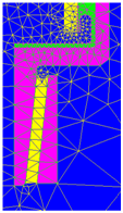
1	The user carries out an initial mesh. It is strongly recommended that the mesh should be carried out by means of the aided mesh. By definition, this mesh is « non-adapted » to the physics of the problem.
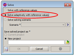
2	To activate the adaptive solver, the user must first open the dialog box Solve which can be found in the Solving menu. Then, select Solve adaptively with reference values.
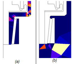
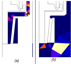
3	For each assigned region, the quality of the mesh is automatically evaluated by means of an error criterion, based on one of the Maxwell equations, appropriated to the studied problem. (a) Epoxy region (b) Air region
4	The mesh is then adapted to the environments where the physics of the problem requires it.
5	The process will be repeated n times until the stop signal criteria are observed.

Here are the different stages of the adaptive solver when the user solves a Flux project by means of a scenario:


Stage	Description	Example
1	The user carries out an initial mesh. It is strongly recommended that the mesh should be carried out by means of the aided mesh. By definition, this mesh is « non-adapted » to the physics of the problem.
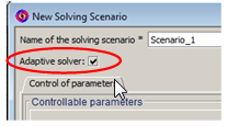
2	To activate the adaptive solver, the user must select Adaptive solver in the scenario that he has created.
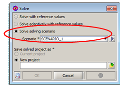
3	The user solves this scenario by opening the dialog box Solve, which exists in the Solving menu and by selecting Solve solving scenario.
4	For each assigned region, the quality of the mesh is automatically evaluated by means of an error criterion, based on one of the Maxwell equations, appropriated to the studied problem. (a) Epoxy region (b) Air region
5	The mesh is adapted then to the environments where the physics of the problem requires it.
6	The process will be repeated n times until the stop signal criteria are observed.

For a simple, efficient use of the adaptive solver, the user can follow the next steps:


Step	Action
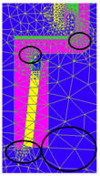
1	Starting from an aided loose mesh such as: Relative deviation = 0.1 Coefficient of relaxation of the line type = 0.9 Coefficient of relaxation of the face type= 0.9
2	In a great majority of cases, two iterations are enough to obtain a mesh adapted to the physics of the problem.