Since version 2026, Flux 3D and Flux PEEC are no longer available.
Please use SimLab to create a new 3D project or to import an existing Flux 3D project.
Please use SimLab to create a new PEEC project (not possible to import an existing Flux PEEC project).
/!\ Documentation updates are in progress – some mentions of 3D may still appear.
Linear solvers: Standard options
General information on linear solvers
A linear system of n equations and n unknowns can be written under the following matrix form:
AX=B
where:
- A is a square matrix of n x n size (with n lines and n columns)
- X is a column vector of size n, representing the system unknowns
- B is a column vector of size n, with known components
To find the solution, i.e. the vector X, a linear solver must be employed. Two types of solvers can be distinguished: the direct and iterative solvers.
The direct solvers follow a process that leads to a very accurate solution but at the cost of several time and memory-expensive operations.
The iterative solvers follow an iterative process that approximates a solution at each iteration. Usually, the process tends to provide a solution closer to the real solution of the linear system from iteration to the next. The process comes with a stopping criterion, depending on the accuracy threshold set for the approximated solution and the maximal number of iterations. Thus, the iterative solver can lead to faster solutions, allowing a predefined inaccuracy threshold.
What solver to use?
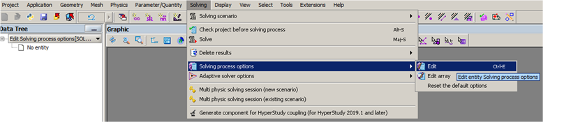
To change the linear solver in use in Altair Flux, go to (see Figure below):
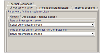
The user can choose between three choices of linear solver:
- Automatic solver,
- Direct solver,
- Iterative solver.
As briefly discussed in the previous section, direct solvers are known to be heavily memory consuming, therefore solving large problems (with a great number of unknowns) will require a larger amount of memory (or RAM) than it would require for iterative solvers. On the other hand, for problems small enough to fit into a given memory amount it can be very handy to use the direct solvers to ensure best results. Moreover, it is very difficult to predict the number of iterations necessary to reach a given accuracy threshold, thus using the direct solver can lead to faster-solving steps. In addition, the direct and the iterative solvers in use are parallel and can take advantage of all the processors available. This is the dilemma the Automatic solver is trying to address. A summary is provided in the Table below:
| Accuracy | Memory | Time | Parallel | ||
|---|---|---|---|---|---|
| Number of nodes | Any | Any | < 500,000 | > 500,000 | Any |
| Direct solver | +++ | --- | ++ | + | YES |
| Iterative solver | ++ | - | + | ++ | YES |
The automatic solver bases its decision to use the Direct or Iterative solver on the application type and the number of unknowns, as summarized in the following Table:
| Dimension | 2D | 3D | |||
|---|---|---|---|---|---|
| Application | Any | Others | Magneto static Integral method | Steady-state AC | |
| Number of nodes | Any | < 500,000 | > 500,000 | Any | Any |
| Solver | Direct | Direct | Iterative | Iterative | Direct |
When a user wants to manually select the solver considering its computational resources, we can advise with the following guidelines:
- For HPC (High Performance Computing) hardware or computers with a great amount of RAM, the Direct solver will be the most suitable choice thanks to its scalability and parallel potential.
- For computers with a low amount of RAM, it would be more advisable to use the Iterative solver for its low memory consumption.
- For 2D problems, the number of unknowns is relatively low, thus Direct solver should deliver better results in terms of solving time.
Adjusting parameters of linear solvers - Standard mode
This section targets advanced users and wants to help understanding what solver parameters do. Let us discuss about the solver options that any user can access. In the standard mode, the solver options are simplified as illustrated in Figure below:
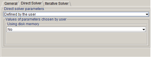
The Direct solver option available consists in using the disk for the solving in addition to the RAM. This option is very useful since it allows extending the amount of usable memory. However, using the disk implies slower operations since disks are significantly slower to compute i/o operations.
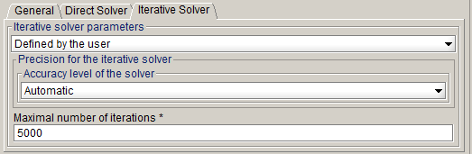
On the right-hand side figure, two options are displayed for the Iterative solver: the precision level (or threshold) and the maximal number of iterations. You can choose between four levels of accuracy: automatic, high, medium and low. Choosing a level for this parameter will deeply depend on your result quality requirement, for predesign simulations one may afford using a low level of precision for example. The lower the level is, the lower the solving time should be. The maximal number of iterations field is straightforward and allow to set a limitation on the solving time. However, be aware that reducing the maximal number of iterations can leads to very inaccurate solutions.
The options discussed above are general options that are applicable to default direct and iterative solvers. Most advanced users who want to select manually the solver to use and not only the type of solver must change their user mode. More informations on Advanced options are available on the page Linear solvers: Advanced options.