B(H) curve
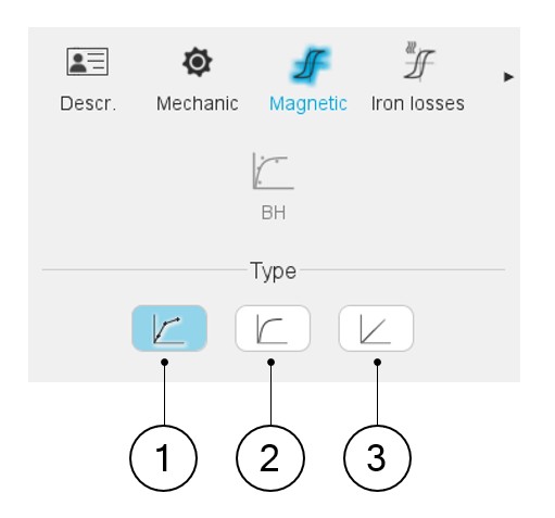
Overview
- Multi-segment B(H) curve: by providing a list of B-H points
- Nonlinear B(H) curve: by providing the three coefficients of the nonlinear analytical model
- Linear B(H) curve: by proving the slope of the B(H) curve
 |
|
|---|---|
| 1 | Multi-segment B(H) curve: by providing a list of B-H points |
| 2 | Nonlinear B(H) curve: by providing the three coefficients of the nonlinear analytical model |
| 3 | Linear B(H) curve: by proving the slope of the B(H) curve |
The resulting relative permeability of the lamination stack is automatically deduced (considering the stacking factor mentioned in the mechanical data).
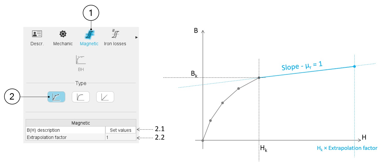
B(H) curve – multi-segments
The B(H) curve is defined with a series of segments. The user must give the list of points (B, H) to define the corresponding segments.
 |
|
|---|---|
| 1 | When editing the properties of an existing material (lamination and solid families), a category is dedicated to the magnetic data. Hence, clicking on the “Magnetic” one can define the B(H) curve. |
| 2 | Selection of the multi-segment model. |
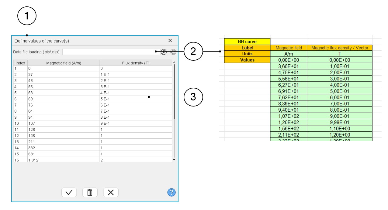
| 2.1 | Set a list of B-H points that describe all the segments for building the B(H) curve. Clicking on this field opens a dialog box in which a table must be filled. See the illustration below. |
| 2.2 | The extrapolation factor allows us to define the slope of the
B(H) curve after the last point given by the user. The aim is to ensure that this slope is equal to 1 (i.e. relative permeability equal to 1). This coefficient is applied to the maximum magnetic field given by the user to define the very last point of the B(H) curve to be considered. The slope equal to 1 is applied to the segment between this point and the last one given by the user, as illustrated in the picture above. |
 |
|
|---|---|
| 1 | Dialog box to describe the B(H) curve with a list of points (B, H). |
| 2 | The building of the multi-segments B(H) curve can be done with an
Excel file. This field helps the user to browse and find the Excel
file to be considered. Note: The format needed
to create the Excel file is illustrated above. |
| 3 | Table in which the list of points must be defined, manually or via an import of an Excel file content. |
It allows to see what the correct format is to be applied for filling the data.
B(H) curve – nonlinear model
- User’s inputs
Table 4. Characterization of the B(H) curve 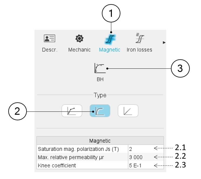
1 When editing the properties of an existing material (lamination and solid families), a category is dedicated to the magnetic data. Hence, clicking on the “Magnetic” one can define the B(H) curve. 2 Selection of the nonlinear analytical B(H) model. The three coefficients of the nonlinear analytical model must be provided. The three main parameters of magnetic characteristic and the analytical formulae to create a B(H) curve are illustrated below. 2.1 The magnetic polarization at saturation (JS) 2.2 The maximum relative magnetic permeability (µr) 2.3 The knee coefficient (a) 3 Another method is possible to define the nonlinear B(H) curve of a material. If the user has measurements or computation points representing the B(H) curve to be modelled, it is possible to import these data to define the corresponding characteristics.
This consists of importing a B(H) curve via an Excel file and identifying the three parameters Js, µr and knee coefficient with an optimization process. See the illustration below
- Define a B(H) curve from experimental data
Here is the process to define the characteristics of the B(H) curve from the importation of a series of points representing the B(H) curve listed in an Excel file.
Table 5. Identification of the B(H) curve characteristics – Fitting data mode 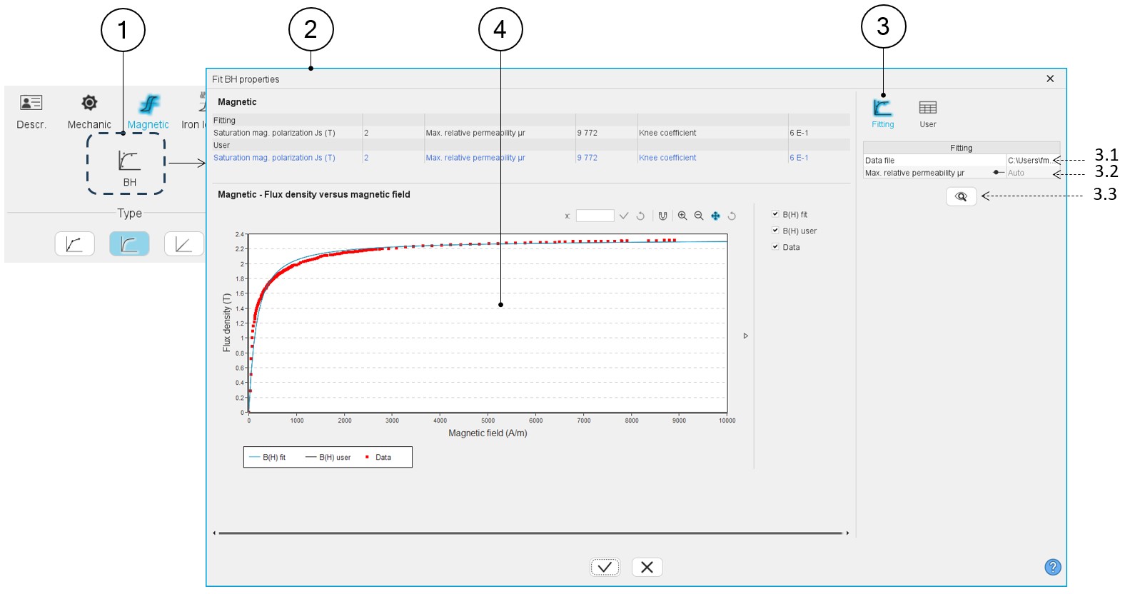
1 Button to fit the B(H) properties. Clicking on it opens the dialog box (2). 2 Dialog box allowing the characterization of the B(H) curve imported from an Excel file. 3 Icon, which corresponds to the option allowing to fit the data in an automatic way. 3.1 Field to browse and to select the path where the Excel file to be imported is stored. See an example of Excel file below. 3.2 In this field, two choices are available: - The automatic mode (Auto): The fitting process is entirely automatic for defining the input parameters for the B(H) curve.
- The setting of the relative permeability: In that case µr is imposed by the user. Hence, the optimization process is run by considering only two variables, Js and a.
3.3 Accept the import of the Excel file data. When importing an Excel file, points representing the B(H) curve are listed. An optimization process automatically computes and displays the corresponding characteristics Js, µr and a. At the same time the curves are displayed (4)
4 Three B(H) curves can be displayed on the graph: - Red points are the imported points (listed in the Excel file)
- The blue curve is the resulting curve computed by the optimization process. This corresponds to the computed characteristics, which is displayed just after the computation.
- The black curve shows modifications induced if the characteristics Js, µr and a are set by the user via the icon “User”. See illustrations below.
Table 6. Identification of the B(H) curve characteristics – User data mode 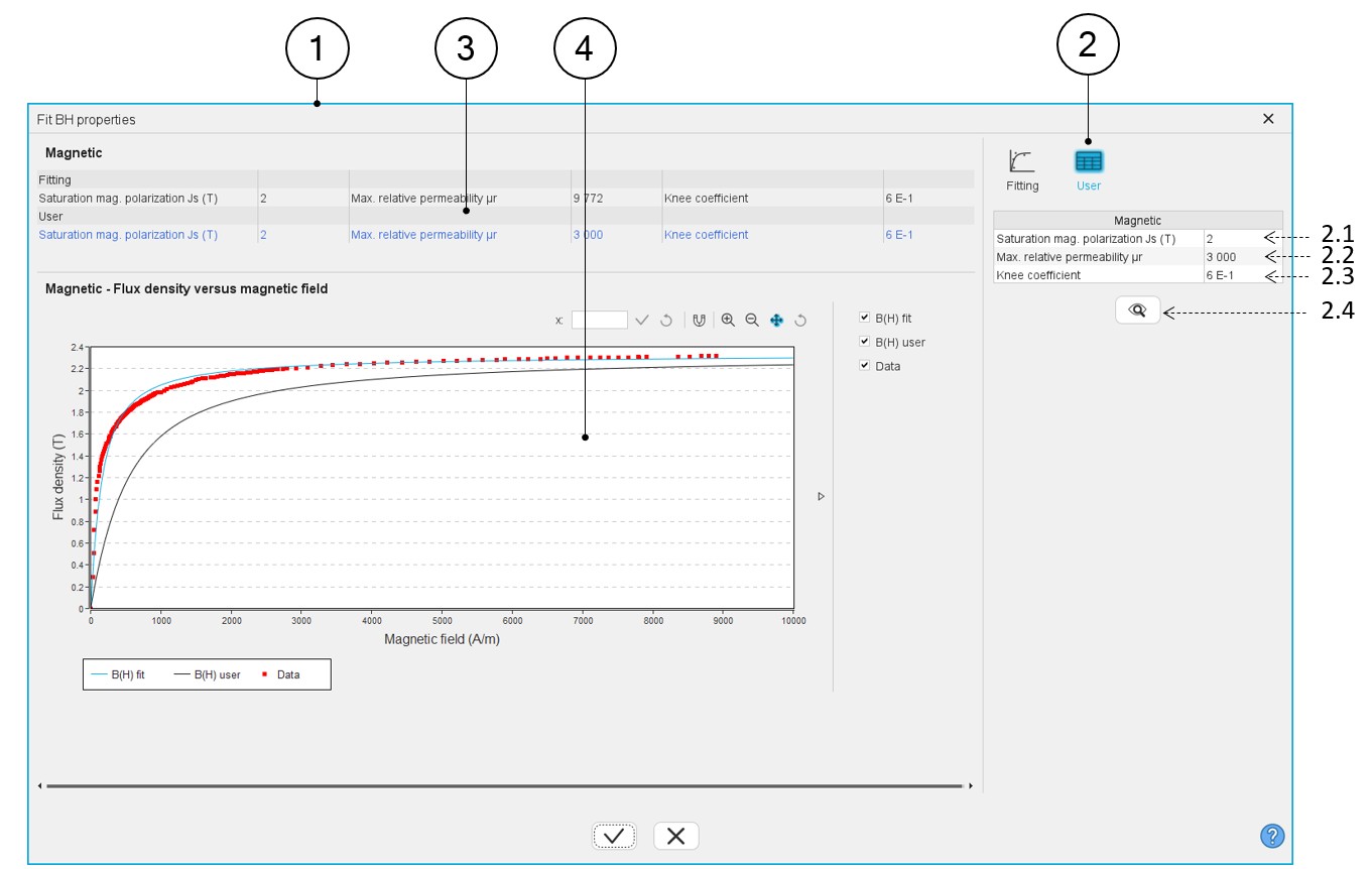
1 Dialog box allowing the characterization of the B(H) curve imported from an Excel file. 2 The user can adjust one or all three main characteristics of the B(H) curve: Js, µr and a. To do so user tab must be selected by clicking on its icon.The resulting modification is directly displayed on the graph (4) and in the magnetic properties (3). 2.1 The magnetic polarization at saturation (Js) 2.2 The maximum relative magnetic permeability (µr) 2.3 The knee coefficient (a) 2.4 Accept the user values modification by clicking this button. 3 The main data of the B(H) curves are displayed: In blue they correspond to the user’s inputs; in black these are the resulting values after the fitting process.
4 Displaying the three B(H) curves: - Red points are the imported points (listed in the Excel file).
- The blue curve is the resulting curve computed by the optimization process. This corresponds to the computed characteristics and is displayed just after the computation.
- The black curve shows modifications induced if the characteristics Js, µr and a are set by the user via the icon “User”.
Example of an Excel file to define the B-H curves parameters.
Figure 1. Example of an Excel file to define the B(H) curve parameters 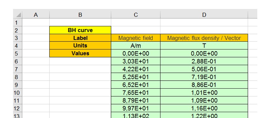
Note: An Excel file “BH_curve_fitting.xls” can be found in the folder …\FluxMotor\Resources\DefaultFiles\Templates\Materials.It allows to see what the correct format is to be applied for filling the data.
- Create a B(H) curve – Main principles
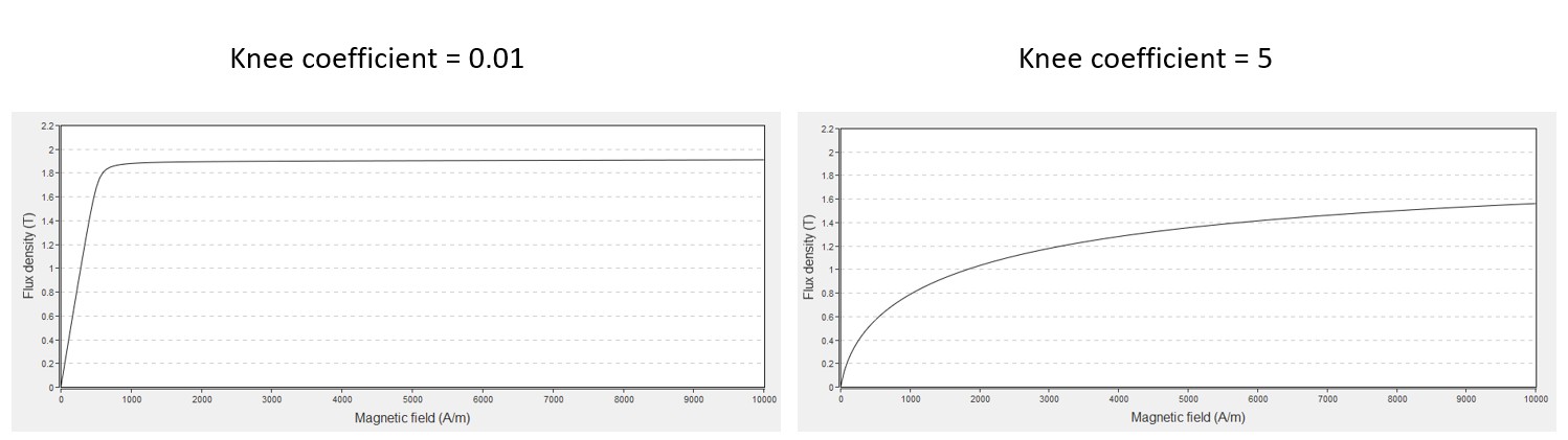
The model consists of a combination of a straight line and a curve. A coefficient allows the adjustment of the knee shape for better approximation of the experimental curve. The corresponding mathematical formula is written as follows:
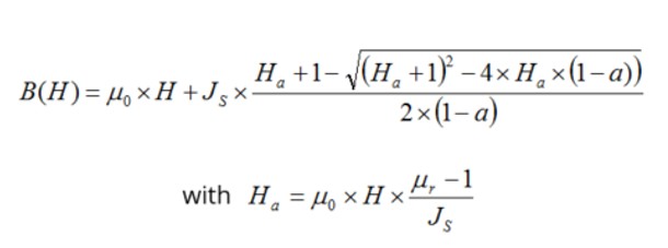
| μ0 | Permeability of vacuum. |
| μr | Initial relative permeability of the material. |
| H | Magnetic field (A/m). |
| Js | Magnetic polarization at saturation (T). |
| a |
Knee coefficient of the curve (a > 0 and a ≠ 1). The smaller coefficient will give, the sharper knee point. |
The impact of the knee coefficient “a” on the shape of the B(H) curve is illustrated in the below figure.
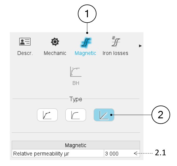
B(H) curve - linear model
 |
|
|---|---|
| 1 | When editing the properties of an existing material (lamination and solid families), a category is dedicated to the magnetic data. Hence, clicking on the “Magnetic” one can define the B(H) curve. |
| 2 | Selection of the linear B(H) model. The linear B(H) characteristic of a lamination is considered, and the slope of the B-H curve must be provided. |
| 2.1 |
Only the relative permeability of the corresponding solid material is given. The resulting relative permeability of the lamination stack is automatically deduced (considering the stacking factor mentioned in the mechanical data). |