Preferences

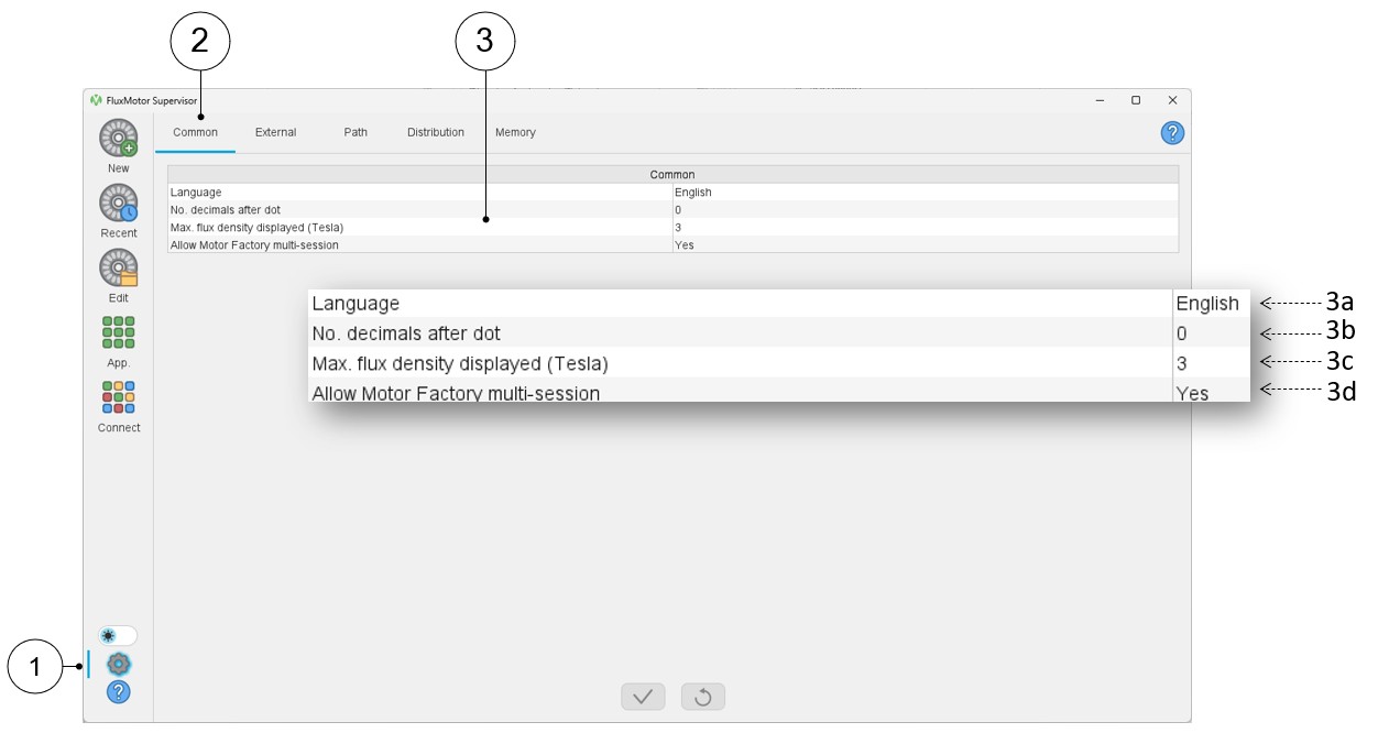
Common user preferences

The different common user preference parameters are listed and illustrated below.

Table 1. FluxMotor – Supervisor – User preferences – Common

1	Access to user’s preferences
2	Selection of the common user preferences
3	List of common user preferences
3a	Choice of language used in FluxMotor application: English is applied by default, but Chinese and Japanese can also be applied in the current version.
3b	Number of decimals to consider after the dot for all the numbers displayed in FluxMotor.
3c	Maximum magnitude of the displayed flux density for visualizing the flux density into the magnetic circuit. The default value is 3 Tesla.
3d	When “Yes” is selected, several Motor Factory sessions can be opened at the same time. “Yes” is set by default.

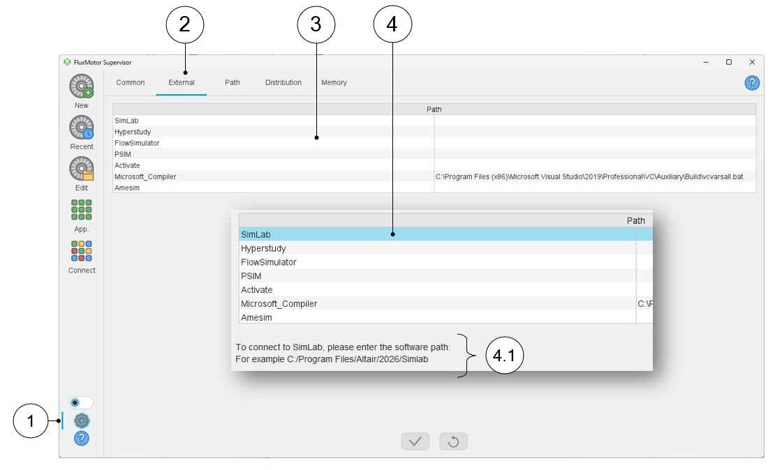
External software preferences

The different External software preference parameters are listed and illustrated below.

Table 2. FluxMotor – Supervisor – User preferences – External software preferences

1	Access to user’s preferences
2	Selection of the external software preferences
3	List of external software where the path can be defined.
4	Definition of the path for the software considered (SimLab in the example).
4.1	Once a software name is selected and highlighted (SimLab in the example), a typical path for the software considered is provided for helping the user.

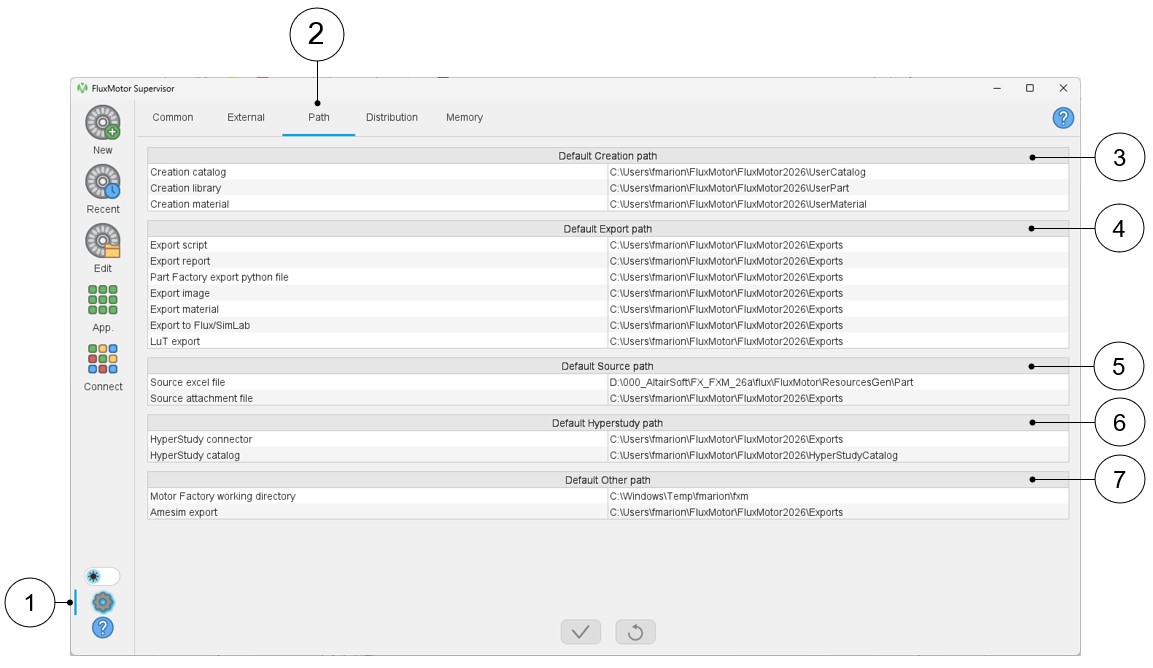
Path preferences

In the path user preferences, the different path types are classified into several sections for better visibility.

Table 3. FluxMotor – Supervisor – User preferences – Default path user preferences

1	Access to user’s preferences
2	Selection of the path user preferences
3	Default Creation path: For storing files generated by applications like Motor Catalog, Part Library or Materials.
4	Default Export path: For storing files that are exported from different applications.
5	Default Source path: For defining the default folder where files can be loaded either for building the part or for adding attachments (Part Library or Motor Catalog).
6	Default HyperStudy path: For defining the default folder where the connectors generated for HyperStudy are stored and where the catalog provided during the HyperStudy process will be stored.
7	Default Other path: Motor Factory working directory and Amesim export folder.

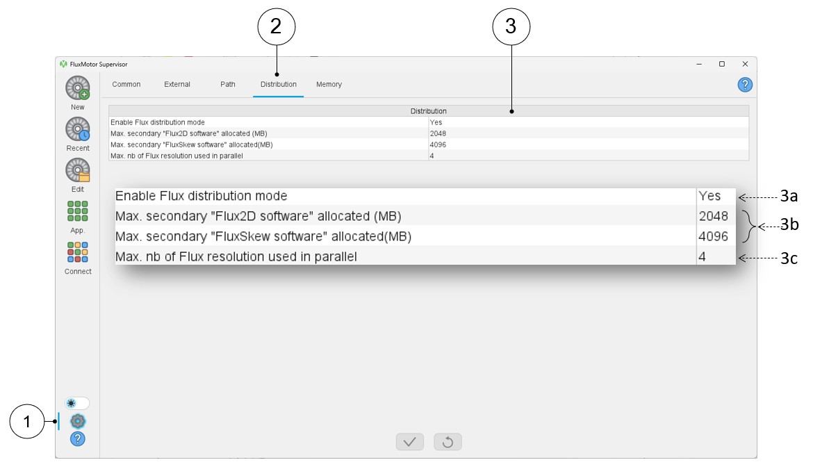
Distribution preferences

In the Distribution user preferences, one can define the Flux distribution mode and the corresponding parameters.

Table 4. FluxMotor – Supervisor – User preferences – Distribution preferences

1	Access to user’s preferences
2	Selection of the distribution preferences
3	Definition of the Flux distribution mode and the corresponding parameters
3a	Enable the Flux solver distribution mode, by default, this option is set to “No”.
3b	Maximum allocated memory for the secondary Flux2D and FluxSkew software when the Flux solver distribution mode is selected. Note: Only static allocated memory can be used. The dynamic memory allocation is not available.
3c	Define the maximum number of cores used by the distribution (See note below)

Enable FLUX distribution mode

1. Introduction

   This section gives information about the establishment of a parametric distribution of the FluxMotor solver, “Flux”, on a single machine. Distributed computing allows the user to save computation time. For example, a test “Scalar Maps” may be automatically distributed if the Flux distribution mode is enabled. In this case, several Flux projects will run at the same time to solve all the required test configurations.

   The main parameter of a distributed computation is the “Maximum number of cores used in distribution mode” (i.e., the number of running Flux in parallel).

   The following topics are covered in this documentation:

   • Principles
   • How to set up a parametric distribution on a single machine?
2. Principles

   The “Flux distribution mode” allows the user to save computation time by parallelizing the finite element (FE) solving of a test.

   Indeed, FE solving is done by parallelizing several independent configurations of an FE problem (such as the value of the stator current) instead of running them sequentially.

   A primary Flux project is launched and controls all the other secondary projects (distribution). The primary project oversees the gathering of all the results obtained during the solving process by all the sub-projects Flux as shown in the figure below:

   
   

   

   
   

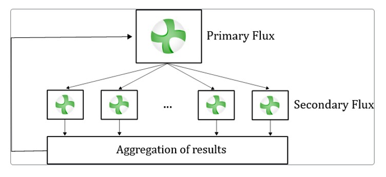
   When the Flux distribution mode is activated, FluxMotor automatically uses it and manages the number of cores used to reduce, as far as possible, the computation time.

   Depending on the number of computation steps, FluxMotor will adapt the number of cores to have at least 10 steps to solve per core.

   In other words, if you select a maximum number of 5 usable cores and solve a test with 25 computation steps ("Characterization - Model - Maps" test with an Id, Iq grid of 5x5), FluxMotor will only distribute the resolution over 2 cores, which is the best configuration according to the FE project to solve.

   Tests that use “Flux distribution mode” are listed in the following table:

   Table 5. Tests that use “Flux distribution mode”

   Machine type	Available with skew	test addressed by Flux distribution
   SM-PM-IR-3Ph SM-PM-OR-3Ph	Yes	Test “Characterization - Model - Maps” Test “Working point - Sine wave - T, N” Test “Performance mapping - Sine wave - Efficiency Map”
   SM-RSM-IR-3Ph	Yes	Test “Characterization - Model - Maps” Test “Performance mapping - Sine wave - Efficiency Map”
   SM-WFISP-IR-3Ph	Yes	Test “Characterization - Model - Maps” Test “Performance mapping - Sine wave - Efficiency Map”
   IM-SQ-IR-3Ph IM-SQ-OR-3Ph	No	Test “Characterization - Model - Scalar Maps” Test “Performance mapping - Sine wave - Efficiency Map scalar U, f” Test “Performance mapping - Sine wave - Efficiency Map scalar U, I”

   An example of the process is shown in the following image for the test “Characterization - Model - Maps” of SM-PM-IR-3Ph:

   
   

   

   
   

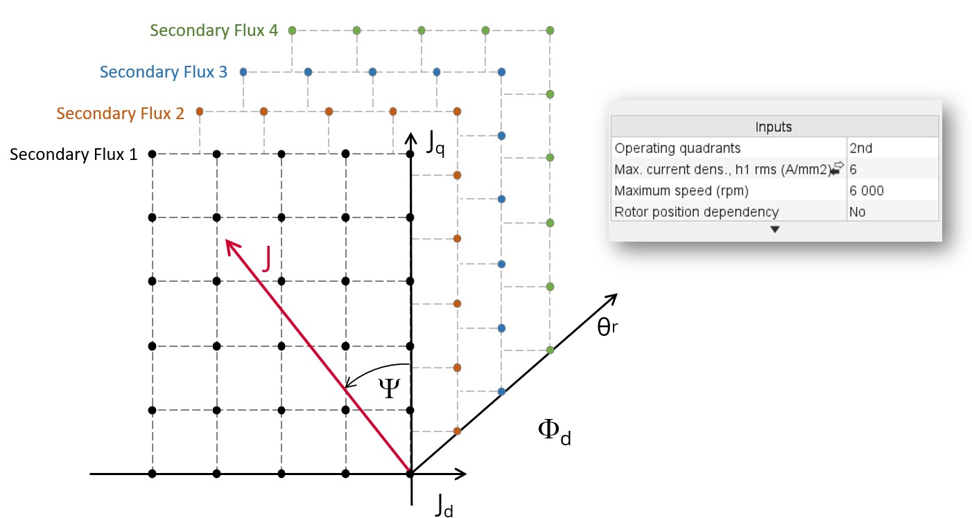
   The following graph shows an example of the solving time versus the number of cores used for a Flux project with 2525 computation steps to solve:

   
   

   

   
   

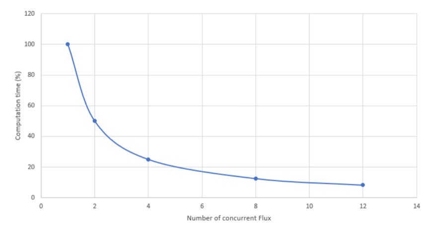
   Note: in FluxMotor:

   • An FE Flux project will be considered of interest for distribution if it contains more than 20 computation steps to solve.
   • From the user's point of view, an FE Flux project’s computation time includes the creation of the FE project, which can take from 45 seconds to several minutes, depending on the case.
   • In most cases, FluxMotor tests involve the sequential solving of several FE Flux projects, and some of these FE Flux projects have no interest in being distributed (less than 20 computation steps).

   According to the previous points, the trend presented in the graph above is therefore not exact in the context of a FluxMotor tests, but it gives a general trend, especially for some tests like “Characterization - Model - Maps” (SM-PM and SM-RSM) or “Characterization - Model - Scalar Maps” (IM-SQ).

3. How to set up a parametric distribution on a single machine?
   In FluxMotor, the Flux distribution mode (number of secondary Flux in parallel) must be set in the user preferences in the section Distribution. It’s just needed to set “Flux distribution mode” to “Yes” and to select the “Maximum number of Flux resolution used in parallel” one wants to use.

   Warning:

   When using the distribution mode, the primary Flux can be used either with dynamic or static memory allocation. However, it is highly recommended to use dynamic memory allocation.

   When using the distribution mode, only the static memory can be used for the secondary Flux. The dynamic memory allocation is not available.

   Table 6. Flux distribution mode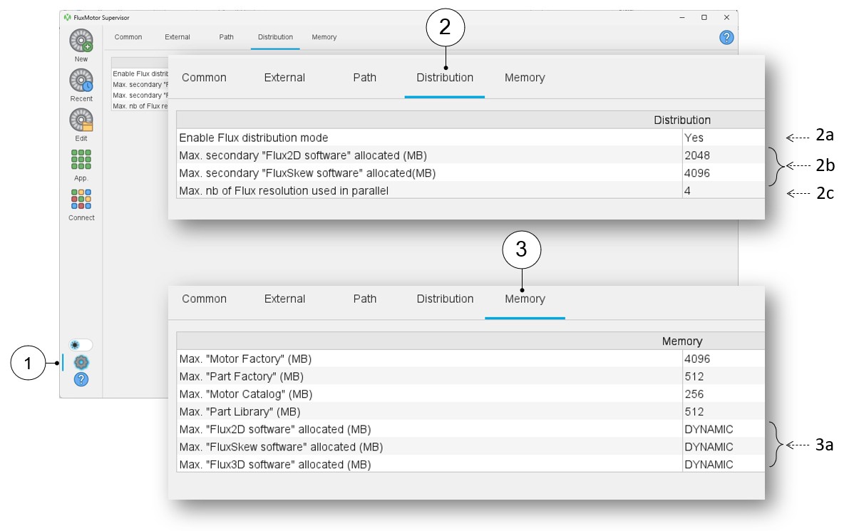

   1	Access to user’s preference
   2	Selection of the distribution preferences
   2a	Field to enable the Flux solver distribution mode. By default, this option is set to “No”.
   2b	Field to set the maximum allocated memory for the secondary Flux (Only static allocated memory can be selected)
   2c	Field to select the maximum number of cores used by the distribution (Maximum number of Flux resolution used in parallel).
   3	Selection of the memory preferences
   3a	Field to set the maximum allocated memory for the primary Flux (Dynamic allocated memory is recommended)

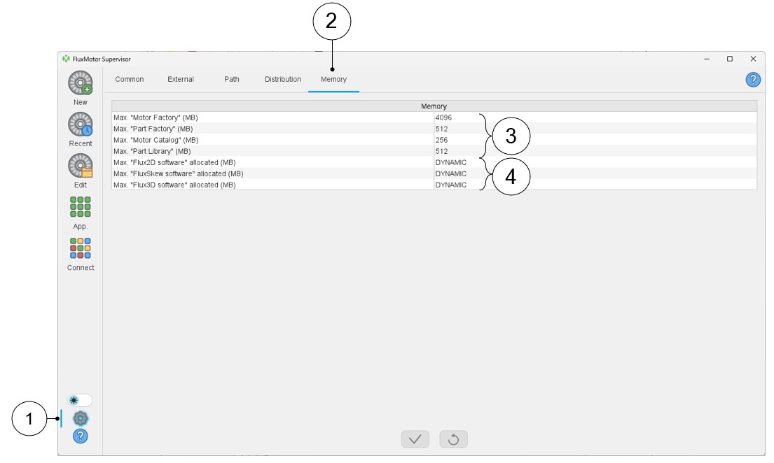
Memory user preferences

In the Memory user preferences, one can define the memory allocation for the different applications used.

Table 7. FluxMotor – Supervisor – User preferences – Memory preferences

1	Access to user’s preferences
2	Selection of the memory preferences
3	Maximum memory allocation for FluxMotor applications. It is recommended to keep default values as far as possible. In case of trouble, consult our support team.
4	Maximum memory allocation for Flux2D and FluxSkew applications. It is recommended to keep default values as far as possible. In case of trouble, consult our support team. Warning: “Maximum Flux3D software allocated (MB)” is a user entry that should not be used. It serves no purpose in this version