h = patch('vertices', vertices_matrix, 'faces', faces_matrix)
h = patch(hAxes, ...)
Inputs
x, y, z
Coordinates of patch vertices.
Type: double | integer
Dimension: vector | matrix
c
Patch color.
Type: char
vertices_matrix
An Mx2 or Mx3 matrix that contains the coordinates of the patch vertices. M is the number of vertices.
Type: double | integer
Dimension: matrix
faces_matrix
An MxN matrix that contains the indices of the vertices of each patch. M is the number
of patches and N is the number of vertices of each patch. NaN may be
used if not all polygons have the same number of vertices (see the Examples
section).
Type: double | integer
Dimension: matrix
hAxes
Axis handle.
Type: double
Dimension: scalar
Outputs
h
Handle of the patch graphics object.
Examples
2D patch plot
example:
clf;
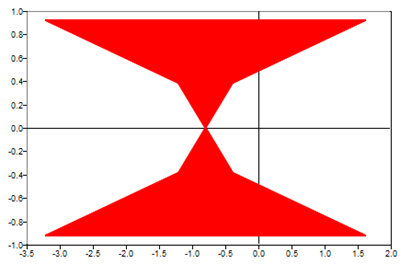
t1 = (1/16:1/8:1) * 2*pi;
t2 = ((1/16:1/8:1) + 1/32) * 2*pi;
x = tan (t1) - 0.8;
y = sin (t1);
h = patch (x',y','r')
Figure 1. 2D patch plot example
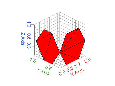
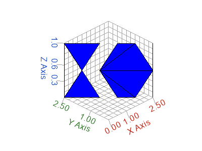
2D patch plot defined by vertices and faces matrices
examples:
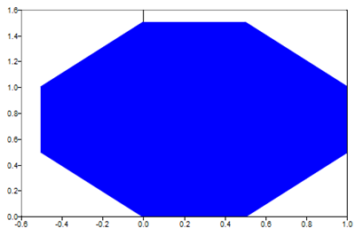
x = [0 0.25 0.5 1 1 0.5 0.25 0 -0.5 -0.5]';
y = [0 0 0 0.5 1 1.5 1.5 1.5 1 0.5]';
verts = [x, y];
figure(1);
% Create one patch which constinst of 10 vertices
faces = [1:10];
h = patch('vertices',verts,'faces',faces);
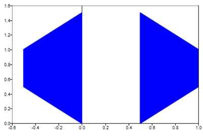
figure(2);
% Create two patches each one consisting of 4 vertices
faces = [3 4 5 6; 8 9 10 1];
h = patch('vertices',verts,'faces',faces);
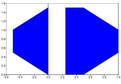
figure(3);
% Create two patches, the first patch consists of 6 vertices,
% the second patch consists of 4 vertices
faces = [2 3 4 5 6 7; 8 9 10 1 NaN NaN];
h = patch('vertices',verts,'faces',faces);
Figure 2. 2D patch plot defined by vertices and faces matrices Figure 3. Create two-2D patches defined by vertices and faces matrices Figure 4. Create two-2D patches that have different number of vertices
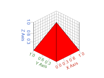
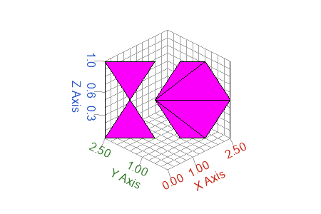
Example of 3D patch plot. Patch faces are triangles:
verts = [0 2.5 0; 1 1.5 0; 1.5 1 0; 2 0.5 0; 2.5 0, 0.5; 2 0.5 1;
1.5, 1 1; 1 1.5 0.5; 1 1.5 1; 0 2.5 1; 0.5 2 0.5];
faces = [1 2 11 NaN NaN NaN; 9 10 11 NaN NaN NaN; 3 4 5 6 7 8];
figure;
h = patch('vertices',verts,'faces',faces);
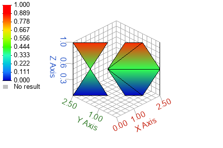
% facecolor = 'interp', the color of each face is defined by interpolating
% the cdata values of its vertices.
% if 'cdata' is not given then the 'zdata' values will be used.
set(h,'facecolor', 'interp');
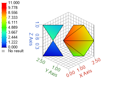
figure;
h = patch('vertices',verts,'faces',faces);
% set a scalar value for each vertex
cdata = [0 1 2 NaN NaN NaN; 3 4 5 NaN NaN NaN; 6 7 8 9 10 11]';
set(h,'cdata', cdata)
set(h,'facecolor', 'interp')
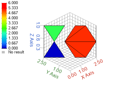
figure;
h = patch('vertices',verts,'faces',faces);
% set a scalar value for each vertex
set(h,'cdata', cdata)
% facecolor = 'flat', the color of each face is defined by the cdata
% value of its first vertex.
set(h,'facecolor', 'flat')
Figure 10. Patch color defined by the 'zdata' value of each vertex Figure 11. Patch color defined by the 'cdata' value of each vertex Figure 12. 'flat' facecolor
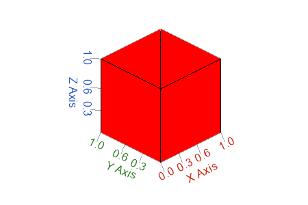
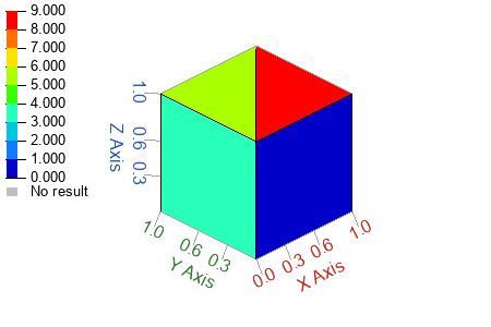
Set color per face:
x = [0 1 1 0; 1 1 0 0; 1 1 0 0; 0 1 1 0];
y = [0 0 1 1; 0 1 1 0; 0 1 1 0; 0 0 1 1];
z = [0 0 0 0; 0 0 0 0; 1 1 1 1; 1 1 1 1];
figure;
h = patch(x,y,z,'r');
% set a scalar value for each face
set(h,'cdata',[0 9 6 4])
set(h,'facecolor', 'flat')
set(gca,'contourtype','discrete')
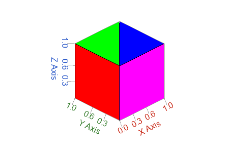
figure;
h = patch(x, y, z, 'r');
% set an rgb color for each face
cdata =[];
cdata(:,:,1) = [255 0 0 255]; % red component
cdata(:,:,2) = [0 0 255 0]; % green component
cdata(:,:,3) = [255 255 0 0]; % blue component
set(h,'cdata',cdata)
set(h,'facecolor', 'flat')
Figure 13. Patch color defined by a scalar value per face Figure 14. RGB color per face