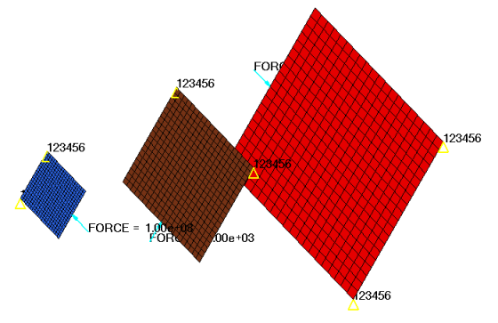
The model used in this tutorial is a rectangular plate with a concentrated force on
one edge and two constraints on the opposite edge. Two other rectangular plates with
a scaled size of 0.6 and 0.3 from the original plate, with forces and boundary
conditions applied in different directions, are also modeled to highlight the
difference between the topology results with and without pattern repetitions.
The objective of this tutorial is to minimize the compliance for the single subcase.
The volume fraction of the design space is limited to 0.3. The design spaces are the
three plates.Figure 1.
Launch HyperMesh and Set the OptiStruct User Profile
Launch HyperMesh.
The User Profile dialog opens.
Select OptiStruct and click
OK.
This loads the user profile. It includes the appropriate template, macro
menu, and import reader, paring down the functionality of HyperMesh to what is relevant for generating models for
OptiStruct.
Import the Model
Click File > Import > Solver Deck.
An Import tab is added to your tab menu.
For the File type, select OptiStruct.
Select the Files icon .
A Select OptiStruct file browser
opens.
Select the no_repeat.fem file you saved
to your working directory.
Click Open.
Click Import, then click Close to
close the Import tab.
Set Up the Optimization
Create Topology Design Variables
From the Analysis page, click optimization.
Click topology.
Select the create subpanel.
In the desvar= field, enter dv1.
Set type: to PSHELL.
Using the props selector, select first.
Click create.
Update the design variable's parameters.
Select the parameters subpanel.
Toggle minmemb off to mindim=, then enter
2.0.
Click update.
Repeat the above steps to create design variables labeled dv2 and dv3 for the
second and third component.
Click return.
Create Optimization Responses
From the Analysis page, click optimization.
Click Responses.
Create the volume fraction response.
In the responses= field, enter Volfrac.
Below response type, select volumefrac.
Set regional selection to total and no
regionid.
Click create.
Create the compliance response.
In the response= field, enter comp.
Below response type, select compliance.
Set regional selection to total and
no regionid.
Click create.
Click return to go back to the Optimization panel.
Create Design Constraints
Click the dconstraints panel.
In the constraint= field, enter volfrac.
Click response = and select Volfrac.
Check the box next to upper bound, then enter
0.3.
Click create.
Click return to go back to the Optimization panel.
Define the Objective Function
Click the objective panel.
Verify that min is selected.
Click response= and select comp.
Using the loadsteps selector, select sub.
Click create.
Click return twice to exit the Optimization panel.
Run the Optimization
From the Analysis page, click OptiStruct.
Click save as.
In the Save As dialog, specify location to write the
OptiStruct model file and enter
no_repeat_opt for filename.
For OptiStruct input decks,
.fem is the recommended extension.
Click Save.
The input file field displays the filename and location specified in the
Save As dialog.
Set the export options toggle to all.
Set the run options toggle to optimization.
Set the memory options toggle to memory default.
Click OptiStruct to run the optimization.
The following message appears in the window at the completion of the
job:
OPTIMIZATION HAS CONVERGED.
FEASIBLE DESIGN (ALL CONSTRAINTS SATISFIED).
OptiStruct also reports error messages if any exist. The
file no_repeat_opt.out can be opened in a
text editor to find details regarding any errors. This file is written to the
same directory as the .fem file.
Click Close.
View the Results Without Pattern Repetition
In this step you will review an Iso Value plot of element densities.
From the OptiStruct panel, click HyperView.
HyperView launches inside of HyperMesh Desktop, and loads the session file
no_repeat_opt.mvw that is linked
with the no_repeat_opt_des.h3d
file.
On the Results toolbar, click to open the Iso Value panel.
Under Result type, select Element Densities(s).
On the Animation toolbar, click to choose the last
iteration from the Simulation list.
Click Apply.
Change the density threshold.
In the Current value field, enter 0.4.
Under Current value, move the slider.
Set Show values to Above.
Under Clipped geometry, select Features and
Transparent.
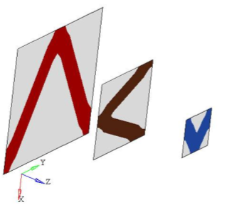
An isosurface plot is displayed. The elements with a density greater
than the value of 0.4 are shown in
color, the rest are transparent.Figure 2.
On the Page Controls toolbar, click the Delete Page icon
to delete the HyperView page.
Figure 3.
Set Up Pattern Repetition
In this step you will define the pattern repetition cards in HyperMesh.
Select nodes.
From the Tool page, click the numbers
panel.
Click nodes > by id, then enter 1329, 66, 6, 46, 507, 447, 487,
928, 892, 948 in the id= field.
Use commas to seperate the values.
Click on.
Click return to exit the Numbers panel.
The selected node's numbers display.
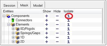
Isolate component collectors.
From the menu bar, click View > Browsers > HyperMesh > Mask to open the Mask Browser.
In the Mask Browser, Isolate column, click 1 to
display only component collectors.
Figure 4.
From the Analysis page, click the optimization
panel.
Click the topology panel.
Select the pattern repetition subpanel.
Create the main DTPL card.
Double-click desvar= and select
dv1.
Set the switch to main.
Toggle from system to coordinates.
Using the first selector, select node ID 6.
Using the second selector, select node ID 46.
Using the third selector, select node ID 1329.
Using the anchor selector, select node ID 66.
Click update.
Create the secondary DTPL card.
Double-click desvar= and select
dv2.
Set the switch to secondary.
Set main= to dv1.
For sx=, enter 0.6; for sy=, enter
0.6; for sz=, enter
1.0.
Toggle from system to coordinates.
Using the first selector, select node ID 447.
Using the second selector, select node ID 487.
Using the third selector, select node ID 1329.
Using the anchor selector, select node ID 507.
Click update.
Create the secondary DTPL card.
Double-click desvar= and select
dv3.
Set the switch to secondary.
Set main= to dv1.
For sx=, enter 0.3; for sy=, enter
0.3; for sz=, enter
1.0.
Toggle from system to coordinates.
Using the first selector, select node ID 892.
Using the second selector, select node ID 928.
Using the third selector, select node ID 1329.
Using the anchor selector, select node ID 948.
Click update.
Click return twice.
You have identified the first DTPL card with ID 1 (on the first
component) as the main, and the DTPL's of ID2 (second component) and
ID 3 (third component) as the secondary, which are dependent on the
DTPL of ID1. The second component is scaled 0.6 in both the x-
and y-axis, while the third component is scaled 0.3 in both the x- and y-axis with
respect to the first component.
Run the Optimization
From the Analysis page, click OptiStruct.
Click save as.
In the Save As dialog, specify location to write the
OptiStruct model file and enter
repeat_opt for filename.
For OptiStruct input decks,
.fem is the recommended extension.
Click Save.
The input file field displays the filename and location specified in the
Save As dialog.
Set the export options toggle to all.
Set the run options toggle to optimization.
Set the memory options toggle to memory default.
Click OptiStruct to run the optimization.
The following message appears in the window at the completion of the
job:
OPTIMIZATION HAS CONVERGED.
FEASIBLE DESIGN (ALL CONSTRAINTS SATISFIED).
OptiStruct also reports error messages if any exist. The
file repeat_opt.out can be opened in a
text editor to find details regarding any errors. This file is written to the
same directory as the .fem file.
Click Close.
View the Results With Pattern Repetition
In this step you will review an Iso Value plot of element densities.
From the OptiStruct panel, click HyperView.
HyperView launches inside of HyperMesh Desktop, and loads the session file
repeat_opt.mvw that is linked
with the repeat_opt_des.h3d
file.
On the Results toolbar, click to open the Iso Value panel.
Under Result type, select Element Densities(s).
On the Animation toolbar, click to choose the last
iteration from the Simulation list.
Click Apply.
Change the density threshold.
In the Current value field, enter 0.38.
Under Current value, move the slider.
Set Show values to Above.
Under Clipped geometry, select Features and
Transparent.
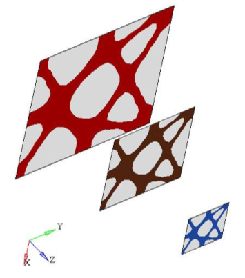
An isosurface plot is displayed. The elements with a density greater
than the value of 0.38 are shown in
color, the rest are transparent.Figure 5.
On the Page Controls toolbar, click the Delete Page icon
to delete the HyperView page.

 .
A Select OptiStruct file browser opens.
.
A Select OptiStruct file browser opens. to open the Iso Value panel.
 to choose the last
iteration from the Simulation list.
to choose the last
iteration from the Simulation list.