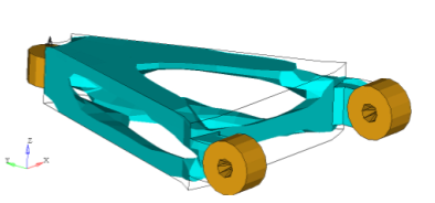
OS-T: 2010 Design Concept for an Automotive Control Arm
In this tutorial you will use OptiStruct's topology optimization functionality to create a design concept for an automotive control arm required to meet performance specifications.
- Objective
- Minimize volume.
- Constraints
- SUBCASE 1. Resultant displacement of the point where loading is applied must be less than 0.05mm.
- Design Variables
- Element density (and corresponding stiffness of the element) of each element in the design space.
Launch HyperMesh and Set the OptiStruct User Profile
-
Launch HyperMesh.
The User Profile dialog opens.
-
Select OptiStruct and click
OK.
This loads the user profile. It includes the appropriate template, macro menu, and import reader, paring down the functionality of HyperMesh to what is relevant for generating models for OptiStruct.
Open the Model
- Click .
- Select the carm.hm file you saved to your working directory.
-
Click Open.
The carm.hm database is loaded into the current HyperMesh session, replacing any existing data.
Set Up the Model
Create the Material
-
In the Model Browser, right-click and select from the context menu.
A default material displays in the Entity Editor.
- For Name, enter Steel.
- Set Card Image to MAT1.
-
Enter the material values next to the corresponding fields.
- For E (Young's Modulus), enter 2.0E5.
- For NU, (Poisson's Ratio), enter 0.3.
- For RHO (Mass Density),
A new material, Steel, has been created. The material uses OptiStruct's linear isotropic material model, MAT1. - Click Close.
Create the Property
-
In the Model Browser, right-click and select from the context menu.
A default property displays in the Entity Editor.
- For Name, enter nondesign_prop.
- Set the Card Image to PSOLID.
-
Assign a material to the property.
- For Material, click .
- In the Select Material dialog, select Steel and click OK.
Assign a Material and Property to the nondesign Component
-
In the Model Browser, Components folder, click nondesign.
The component displays in the Entity Editor.
- For Property, click . In the Select Property dialog, select nondesign_prop and click OK.
- Repeat the above steps to assign the design_prop property to the design component.
Apply Loads and Boundary Conditions
Create Load Collectors
-
In the Model Browser, right-click and select from the context menu.
A default load collector displays in the Entity Editor.
- For Name, enter SPC.
- Click Color and select a color from the color palette.
- Set Card Image to None and click Close.
- Repeat the above steps to create load collectors named Brake, Corner, and Pothole.
Apply Constraints
- From the Model Browser, Load Collectors folder, right-click on SPC and select Make Current from the context menu.
- From the Analysis page, click constraints.
- Set the Load type to SPC.
-
Create the first constraint.
A constraint is created. A constraint symbol (triangle) appears at the selected node. The number 123 is displayed beside the constraint symbol, indicating that dof1, dof2 and dof3 are constrained.
Figure 2. Constrain dof1, dof2 and dof3 at One End of the Bushing 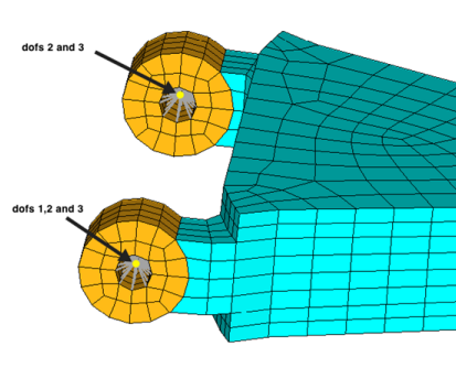
-
Create the second constraint.
- Using the nodes selector, select the node at the other end of the bushing.
- Select the degrees of freedom, dof2 and dof3; unselect all others.
- Click create.
Figure 3. Constrain dof2 and dof3 at the Other End of the Bushing 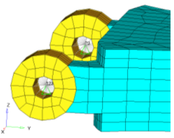
-
Create the third constraint.
Figure 4. Constrain dof3 on Node ID 3239 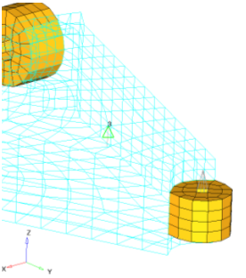
- Click return.
Apply Forces to the Brake, Corner and Pothole Loadcases
- From the Analysis page, click forces.
-
Apply a force to the Brake load case.
- From the Model Browser, Load Collectors folder, right-click on Brake and select Make Current from the context menu.
- Double-click the nodes and select by id, then enter 2699.
- In the magnitude= field, enter 1000.
- Set the vector selector to x-axis.
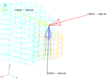
- Click create.
An arrow, pointing in the x direction, appears at the selected node.Tip: For better visualization of the forces, in the uniform size= field, enter 100. -
Apply a force to the Corner load case.
- From the Model Browser, Load Collectors folder, right-click on Corner and select Make Current from the context menu.
- Double-click the nodes and select by id, then enter 2699.
- In the magnitude= field, enter 1000.
- Set the vector selector to y-axis.
- Click create.
An arrow, pointing in the y direction, appears at the selected node. -
Apply a force to the Pothole load case.
- From the Model Browser, Load Collectors folder, right-click on Pothole and select Make Current from the context menu.
- Double-click the nodes and select by id, then enter 2699.
- In the magnitude= field, enter 1000.
- Set the vector selector to z-axis.
- Click create.
An arrow, pointing in the z direction, appears at the selected node. - Click return to go back to the Analysis page.
Create Load Steps
- In the Model Browser, right-click and select from the context menu.
- For Name, enter Brake.
- Set Analysis type to linear static.
-
Define SPC.
-
For SPC, click Unspecified >
 to open Advanced Selection.
- In the dialog, select SPC and click OK.
-
For SPC, click Unspecified >
- In Subcase Options, select .
-
For LOAD, click Unspecified > to open Advanced Selection.
- In the dialog, select Brake and click OK.
-
Repeat the above steps to create load steps named Corner and Pothole.
- For the Corner load step, set SPC to SPC and LOAD to Corner.
- For the Pothole load step, set SPC to SPC and LOAD to Pothole.
Set Up the Optimization
Create Topology Design Variables
- From the Analysis page, click optimization.
- Click topology.
- Select the create subpanel.
- In the desvar= field, enter design_prop.
- Set type: to PSOLID.
- Using the props selector, select design_prop.
- Click create.
- Click return.
Create Optimization Responses
- From the Analysis page, click optimization.
- Click Responses.
-
Create the volume response, which defines the volume fraction of the design
space.
- In the responses= field, enter vol.
- Below response type, select volume.
- Set regional selection to total and no regionid.
- Click create.
-
Create the displacement response.
- Click return to go back to the Optimization panel.
Create Constraints on Displacement Responses
- Click the Dconstraints panel.
-
Create the first constraint.
- In the constraint= field, enter constr1.
- Check the box next to upper bound, then enter 0.05.
- Click response= and select disp1.
- Using the loadsteps selector, select Brake.
- Click create.
-
Create the second constraint.
- In the constraint= field, enter constr2.
- Check the box next to upper bound, then enter 0.02.
- Click response= and select disp1.
- Using the loadsteps selector, select Corner.
- Click create.
-
Create the third constraint.
- In the constraint= field, enter constr3.
- Check the box next to upper bound, then enter 0.05.
- Click response= and select disp1.
- Using the loadsteps selector, select Pothole.
- Click create.
- Click return to go back to the Optimization panel.
Define the Objective Function
- Click the objective panel.
- Verify that min is selected.
- Click response= and select vol.
- Click create.
- Click return twice to exit the Optimization panel.
Check the Optimization Problem
- From the Analysis page, click the OptiStruct panel.
- Click save as.
-
In the Save As dialog, specify location to write the
OptiStruct model file and enter
carm_complete for filename.
For OptiStruct input decks, .fem is the recommended extension.
-
Click Save.
The input file field displays the filename and location specified in the Save As dialog.
- Set the export options toggle to all.
- Set the run options toggle to check.
- Set the memory options toggle to memory default.
- Click OptiStruct to launch the OptiStruct job.
- Is the optimization problem set up correctly?
- Refer to the Optimization Problem Parameters section.
- Is the objective function set up correctly?
- Refer to the Problem Parameters section.
- Are the constraints set up correctly?
- Refer to the Optimization Problem Parameters section.
- What is the recommended amount of RAM for an In-Core solution?
- Refer to the Memory Estimation Information section.
- Is there enough disk space to run the optimization?
- Refer to the Disk Space Estimation Information section.
Run the Optimization
- From the Analysis page, click OptiStruct.
- Click save as.
-
In the Save As dialog, specify location to write the
OptiStruct model file and enter
carm_complete for filename.
For OptiStruct input decks, .fem is the recommended extension.
-
Click Save.
The input file field displays the filename and location specified in the Save As dialog.
- Set the export options toggle to all.
- Set the run options toggle to optimization.
- Set the memory options toggle to memory default.
-
Click OptiStruct to run the optimization.
The following message appears in the window at the completion of the job:
OptiStruct also reports error messages if any exist. The file carm_complete.out can be opened in a text editor to find details regarding any errors. This file is written to the same directory as the .fem file.OPTIMIZATION HAS CONVERGED. FEASIBLE DESIGN (ALL CONSTRAINTS SATISFIED). - Click Close.
- carm_complete.res
- HyperMesh binary results file.
- carm_complete.HM.comp.cmf
- HyperMesh command file used to organize elements into components based on their density result values. This file is only used with OptiStruct topology optimization runs.
- carm_complete.out
- OptiStruct output file containing specific information on the file setup, the setup of the optimization problem, estimates for the amount of RAM and disk space required for the run, information for all optimization iterations, and compute time information. Review this file for warnings and errors that are flagged from processing the carm_complete.fem file.
- carm_complete.sh
- Shape file for the final iteration. It contains the material density, void size parameters and void orientation angle for each element in the analysis. This file may be used to restart a run.
- carm_complete.hgdata
- HyperGraph file containing data for the objective function, percent constraint violations, and constraint for each iteration.
- carm_complete.oss
- OSSmooth file with a default density threshold of 0.3. You may edit the parameters in the file to obtain the desired results.
- carm_complete.stat
- Contains information about the CPU time used for the complete run and also the break-up of the CPU time for reading the input deck, assembly, analysis, convergence, and so on.
- carm_complete.his_data
- The OptiStruct history file containing iteration number, objective function values and percent of constraint violation for each iteration.
- carm_complete.HM.ent.cmf
- HyperMesh command file used to organize elements into entity sets based on their density result values. This file is only used with OptiStruct topology optimization runs.
- carm_complete.html
- HTML report of the optimization, giving a summary of the problem formulation and the results from the final iteration.
View the Results
Element density results are output to the carm_complete_des.h3d file from OptiStruct for all iterations. In addition, Displacement and Stress results are output for each subcase for the first and last iterations by default into carm_complete_s#.h3d files, where # specifies the sub case ID.
View the Deformed Structure
-
From the OptiStruct panel, click HyperView.
HyperView launches inside of HyperMesh Desktop, and loads all three .h3d files in a different page of HyperView. The analysis results are available in pages 2, 3, and 4. The first page contains the optimization results.
-
In the top, left of the application click
 to
move to the third page.
The second page has the results from the carm_complete_s1.h3d file. The name of the page is displayed as Subcase 1 - Brake to indicate that the results correspond to subcase 1.
to
move to the third page.
The second page has the results from the carm_complete_s1.h3d file. The name of the page is displayed as Subcase 1 - Brake to indicate that the results correspond to subcase 1. -
From the Animation toolbar, set the animation mode to linear (
 ).
).
-
Define contour settings.
-
From the Results toolbar, click
 to open the Contour panel.
- Under Result type, select Displacement [v] and Mag.
- Click Apply to display the displacement contour.
-
From the Results toolbar, click
-
Define the deformed shape settings.
-
From the Results toolbar, click
 to open the Deformed panel.
A deformed plot of your model with displacement contour should be visible, overlaid on the original undeformed mesh. -
From the Results toolbar, click
-
From the Animation toolbar, click
 (Start/Pause) to animate the model.
A deformed animation for the first subcase (brake) should be displayed.
Analyze the following:- In what direction is the load applied for the first subcase?
- Which nodes have degrees of freedom constrained?
- Does the deformed shape look correct for the boundary conditions applied to the mesh?
-
In the Results Browser, select Iteration 18.
The contour now shows the displacement results for Subcase 1 (brake) and iteration 18 which corresponds to the end of the optimization iterations.
Figure 6. 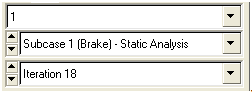
-
From the Animation toolbar, click
 to
stop the animation.
to
stop the animation.
-
In the top, right of the application click to
move to the third page.
The third page has results loaded from carm_complete_s2.h3d file. The name of the page is displayed as Subcase 2 - corner to indicate that the results correspond to subcase 2.
-
Repeat the above steps to display the displacement contours and deformed shape
of the model for the second subcase.
Analyze the following:
- In what direction is the load applied for the second subcase?
- Which nodes have degrees of freedom constrained?
- Does the deformed shape look correct for the boundary conditions applied to the mesh?
- Similarly, review the displacements and deformation for subcase 3 (pothole).
Review the Contour Plot of the Density Results
-
In the top, right of the application click
 to
go back to the Design History page.
to
go back to the Design History page.
-
Define contour settings.
-
On the Results toolbar, click to open the Contour panel.
Notice: The Result type is set to Element Densities (s) and Density. This should be the only result type in the carm_complete_des.h3d file.
The density contour displays. The contour is all blue because your results are on the first design step or Iteration 0. -
On the Results toolbar, click
-
In the Results Browser, select Iteration 18.
Each element of the model is assigned a legend color, indicating the density of each element for the selected iteration.
Analyze the following:- Have most of your elements converged to a density close to 1 or 0?
- If there are many elements with intermediate densities, the DISCRETE parameter may need to be adjusted. The DISCRETE parameter (set in the opti control panel on the optimization panel) can be used to push elements with intermediate densities towards 1 or 0 so that a more discrete structure is given.
- Does the max= field show 1.0e+00?
- In this case, it is.
View an Iso Value Plot of Element Densities
- From the menu bar, click .
- In the Iso panel, set Result type to Element Densities (s).
- Click Apply.
-
Change the density threshold.
- In the Current value field, enter 0.15.
- Under Current value, move the slider.
The Iso value in the modeling window updates interactively when you enter a new value or move the slider. This feature is useful when you want to get a better look at the material layout and the load paths from OptiStruct.Figure 7.