OS-T: 2000 Design Concept for a Structural C-Clip

In this tutorial you will perform a topology optimization on a model to create a new topology for the structure, removing any unnecessary material. The resulting structure is lighter and satisfies all design constraints.

Before you begin, copy the file(s) used in this tutorial to your working directory.

cclip.hm

The topology optimization technique yields a new design and optimal material distribution. Topology optimization allows designers to start with a design that already has the advantage of optimal material distribution and is ready for design fine tuning with shape or size optimization.

The optimization problem for this tutorial is stated as:

Objective: Minimize volume fraction.
Constraints: Translation in the y-axis for node A < 0.07mm.; Translation in the y-axis at node B > -0.07mm.
Design variables: The density of each element in the design space.

Launch HyperMesh and Set the OptiStruct User Profile

Launch HyperMesh.
The User Profile dialog opens.
Select OptiStruct and click OK.
This loads the user profile. It includes the appropriate template, macro menu, and import reader, paring down the functionality of HyperMesh to what is relevant for generating models for OptiStruct.

Open the Model

Click File > Open > Model.
Select the cclip.hm file you saved to your working directory.
Click Open.
The cclip.hm database is loaded into the current HyperMesh session, replacing any existing data.

Set Up the Model

Create the Material

In the Model Browser, right-click and select Create > Material from the context menu.
A default material displays in the Entity Editor.
For Name, enter steel.
Set Card Image to MAT1.
Enter the material values next to the corresponding fields.
1. For E (Young's Modulus), enter 2.1E5.
2. For NU, (Poisson's Ratio), enter 0.3.
3. For RHO (Mass Density),

A new material, steel, has been created. The material uses OptiStruct's linear isotropic material model, MAT1.

Create the Property

In the Model Browser, right-click and select Create > Property from the context menu.
A default property displays in the Entity Editor.
For Name, enter prop_shell.
Set Card Image to PSHELL.
Enter the property values next to the corresponding fields.
An empty Value field indicates that it is turned off. To edit these properties, click on the blank Value fields next to them and enter the required values.
1. For Material, click Unspecified > Material. In the Select Material dialog, select steel and click OK.
2. For T (thickness of the plate), enter 1.0.

A new property, prop_shell, has been created as a 2D PSHELL. Material information is also linked to this property.

Assign a Material and Property to the comp_shell Component

In the Model Browser, Components folder, click comp_shell.
The component displays in the Entity Editor.
For Property, click Unspecified > Property. In the Select Property dialog, select prop_shell and click OK.

Apply Loads and Boundary Conditions

Create Load Collectors

In the Model Browser, right-click and select Create > Load Collector from the context menu.
A default load collector displays in the Entity Editor.
For Name, enter constraints.
Click Color and select a color from the color palette.
Set Card Image to None.
Create another load collector.
1. For Name, enter forces.
2. For Card Image, select None.

Create Constraints

In this step you will create SPC constraints and assign them to the Constraints load collector.

From the Model Browser, Load Collectors folder, right-click on Constraints and select Make Current from the context menu.
From the Analysis page, click constraints.
Create the first constraint.
1. Using the nodes selector, select the node indicated in Figure 1.
2. Select the degree of freedom, dof3; unselect all others.
3. Click create.
Figure 1.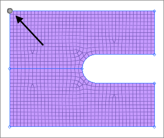
Create the second constraint.
1. Using the nodes selector, select the node indicated in Figure 2.
2. Select the degrees of freedom, dof1 - dof3; unselect all others.
3. Click create.
Figure 2.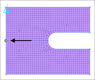
Create the third constraint.
1. Using the nodes selector, select the node indicated in Figure 3.
2. Select the degree of freedom, dof2; unselect all others.
3. Click create.
Figure 3.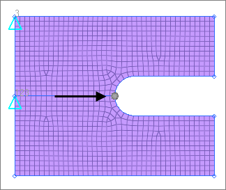
Click return.

Create Forces

In this step, you will load the structure with two opposing forces of 100.0 N at the opposite tips of the opening of the c-clip.

From the Model Browser, Load Collectors folder, right-click on Forces and select Make Current from the context menu.
From the Analysis page, click forces.
Create a force at the top of the opening of the c-clip.
1. Using the nodes selector, select the node at the top of the opening of the clip.
2. In the magnitude= field, enter 100.
3. Set the vector selector to y-axis.
4. Click create.
Figure 4.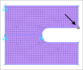
Create a force at the bottom of the opening of the c-clip.
1. Using the nodes selector, select the node at the bottom of the opening of the clip.
2. In the magnitude= field, enter -100.
3. Set the vector selector to y-axis.
4. Click create.
Figure 5.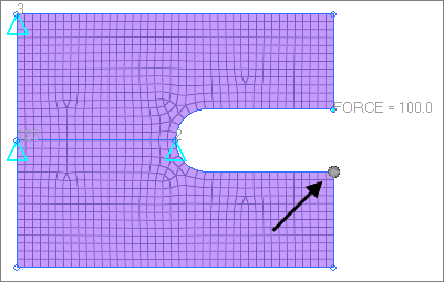
To provide a separation between the arrows, enter 7 in the uniform size= field.

Figure 6.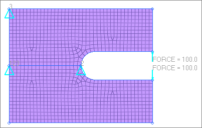
Click return to go back to the Analysis page.

Create Load Steps

In the Model Browser, right-click and select Create > Load Step from the context menu.
For Name, enter opposing forces.
Set Analysis type to linear static.
Define SPC.
1. For SPC, click Unspecified > Loadcol.
2. In the Select Loadcol dialog, select constraints and click OK.
Define LOAD.
1. For LOAD, click Unspecified > Loadcol.
2. In the Select Loadcol dialog, select forces and click OK.

Submit the Job

A linear static analysis of this C-clip is performed prior to the definition of the optimization process. An analysis identifies the responses of the structure before optimization to ensure that constraints defined for the optimization are reasonable.

From the Analysis page, click the OptiStruct panel.

Figure 7. Accessing the OptiStruct Panel
Click save as.
In the Save As dialog, specify location to write the OptiStruct model file and enter cclip_complete for filename.
For OptiStruct input decks, .fem is the recommended extension.
Click Save.
The input file field displays the filename and location specified in the Save As dialog.
Set the export options toggle to all.
Set the run options toggle to analysis.
Set the memory options toggle to memory default.
Clear the options field.
Click OptiStruct to launch the OptiStruct job.

If the job is successful, new results files should be in the directory where the cclip_complete.fem was written. The cclip_complete.out file is a good place to look for error messages that could help debug the input deck if any errors are present.

View the Results

From the OptiStruct panel, click HyperView.
HyperView launches the cclip.mvw file which loads the model and the results files.
On the Results toolbar, click to open the Contour panel.
Under Result type, select Displacement(v) and Y.
Click Apply.

Figure 8. Contour of Y Displacements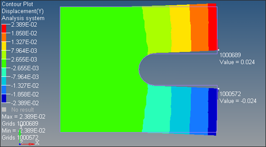
Verify if the values are equivalent to those in Figure 8.
From the Page Control toolbar, click the page delete icon to delete the HyperView page.

Figure 9.

HyperView closes.
Click return to exit the panel.

Set Up the Optimization

The finite element model, consisting of shell elements, element properties, material properties, and loads and boundary conditions has been defined. Now a topology optimization will be performed with the goal of minimizing the amount of material to be used. Typically, removing the material in an existing volume with the same loads and boundary conditions makes the model less stiff and more prone to deformation. Therefore, you need to track the displacements (which represent the stiffness of the structure) and constrain the optimization process such that the least material necessary is used and overall stiffness is also achieved.

The forces in the structure are applied on the outer nodes of the opening of the clip, making those two nodes critical locations in the mesh where the maximum displacement is likely to occur. In this tutorial, you will apply a displacement constraint on the nodes so that they would not displace more than 0.07 in the y-axis.

Create Topology Design Variables

From the Analysis page, click optimization.
Click topology.
Select the create subpanel.
In the desvar= field, enter d_shell.
Set type: to PSHELL.
Using the props selector, select prop_shell.
Verify that the base thickness is 0.0.

A value of 0.0 implies that the thickness at a specific element can go to zero, and therefore becomes a void.
Click create.
Click return.

Create Optimization Responses

From the Analysis page, click optimization.
Click Responses.
Create the volume fraction response.
1. In the responses= field, enter volfrac.
2. Below response type, select volumefrac.
3. Set regional selection to total and no regionid.
4. Click create.
Create the displacement response.
1. In the response= field, enter upperdis.
2. Below response type, select static displacement.
3. Set the displacement type to dof2.
  
  dof1, dof2, dof3
  
  Translation in the X, Y, and Z directions.
  
  dof4, dof5, dof6
  
  Rotation about the X, Y, and Z axes.
  
  total disp
  
  Resultant of the translational displacements in x, y, and z directions.
  
  total rotation
  
  Resultant of the rotational displacements in x, y, and z directions.
4. Click create.
Figure 10.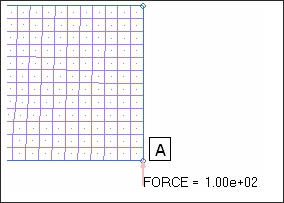
Create another displacement response, named lowerdis. Using the nodes selector, select the node labeled B, on the lower opening of the c-clip.

Figure 11.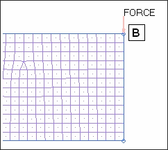
Click return to go back to the Optimization panel.

Create Constraints on Displacement Responses

In this step, the upper and lower bound constraint criteria for this analysis will be set.

Click the Dconstraints panel.
Create the upper bound constraint.
1. In the constraint= field, enter c_upper.
2. Check the box next to upper bound, then enter 0.07.
3. Click response= and select upperdis.
4. Using the loadsteps selector, select opposing forces.
5. Click create.
Create the lower bound constraint.
1. In the constraint= field, enter c_lower.
2. Check the box next to lower bound, then enter -0.07.
3. Click response= and select lowerdis.
4. Using the loadsteps selector, select opposing forces.
5. Click create.
Click return to go back to the Optimization panel.

Define the Objective Function

Click the objective panel.
Verify that min is selected.
Click response= and select volfrac.
Click create.
Click return twice to exit the Optimization panel.

Create the SCREEN Card

The SCREEN control card enables OptiStruct to output the optimization iterations to the output window.

From the Analysis page, click control cards.
In the Card Image dialog, click SCREEN.
Click return.
Click return.

Run the Optimization

From the Analysis page, click OptiStruct.
Click save as.
In the Save As dialog, specify location to write the OptiStruct model file and enter cclip_complete for filename.
For OptiStruct input decks, .fem is the recommended extension.
Click Save.
The input file field displays the filename and location specified in the Save As dialog.
Set the export options toggle to all.
Set the run options toggle to optimization.
Set the memory options toggle to memory default.
Click OptiStruct to run the optimization.
The following message appears in the window at the completion of the job:
```
OPTIMIZATION HAS CONVERGED.
FEASIBLE DESIGN (ALL CONSTRAINTS SATISFIED).
```
OptiStruct also reports error messages if any exist. The file cclip_complete.out can be opened in a text editor to find details regarding any errors. This file is written to the same directory as the .fem file.
Click Close.

The default files that get written to your run directory include:

cclip_complete.hgdata: HyperGraph file containing data for the objective function, percent constraint violations, and constraint for each iteration.
cclip_complete.HM.comp.tcl: HyperMesh command file used to organize elements into components based on their density result values. This file is only used with OptiStruct topology optimization runs.
cclip_complete.oss: OSSmooth file with a default density threshold of 0.3. You may edit the parameters in the file to obtain the desired results.
cclip_complete.out: OptiStruct output file containing specific information on the file setup, the setup of the optimization problem, estimates for the amount of RAM and disk space required for the run, information for all optimization iterations, and compute time information. Review this file for warnings and errors that are flagged from processing the cclip_complete.fem file.
cclip_complete.res: HyperMesh binary results file.
cclip_complete.sh: Shape file for the final iteration. It contains the material density, void size parameters and void orientation angle for each element in the analysis. This file may be used to restart a run.
cclip_complete.stat: Contains information about the CPU time used for the complete run and also the break-up of the CPU time for reading the input deck, assembly, analysis, convergence, and so on.
cclip_complete_hist.mvw: Contains the iteration history of the objective, constraints, and the design variables. It can be used to plot curves in HyperGraph, HyperView, and MotionView.
cclip_complete.h3d: HyperView binary results file.

View the Results

Element density results are output to the cclip_complete_des.h3d file from OptiStruct for all iterations. In addition, Displacement and Stress results are output for each subcase for the first and last iterations by default into cclip_complete_s#.h3d files, where # specifies the sub case ID.

View an Iso Value Plot of Element Densities

An Iso Value plot provides information about element densities. Iso Value retains all of the elements at and above a certain density threshold. You should pick a density threshold that provides the structure that suits your needs.

From the OptiStruct panel, click HyperView.
HyperView launches inside of HyperMesh Desktop, and opens the session file cclip_complete.mvw which contains two pages with the results from two files.

Page 2

Displays the file cclip_complete_des.h3d, which contains the Optimization history results (element density).

Page 3

Displays the cclip_complete_s1.h3d, which contains the Subcase 1 results; initial and final (displacement stress).
Verify that you are on page 2.
In the Results Browser, under the load case section, select Design and the last iteration listed to review the optimized iteration result.

Figure 12.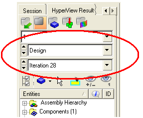
On the Standard Views toolbar, click XY Top Plane View to set the correct view.
From the menu bar, click Results > Plot > Iso.
In the panel area, set Result type to Element Densities.
Click Apply.
In the Current value field, enter 0.3.
Under Current value, move the slider to change the density threshold.
Use this tool to get a better look at the material layout and the load paths from OptiStruct.

The iso value in the modeling window update interactively when you scroll to a new value.

Figure 13. Iso Value Plot of Element Densities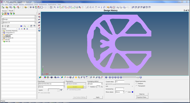

Compare Original Static Contour to Optimized Material Layout

In HyperView, click to go to page 3.
The cclip_complete_s1.h3d file displays, which contains the static subcase results for the first and last iteration steps.
On the Page Controls toolbar, from the Page Window Layout drop-down, click to divide the page into two vertical windows.
On the Standard Views toolbar, click XY Top Plane View to set the correct view.
From the menu bar, click Results > Plot > Contour.
Under Result type, select Displacement and Y.
Click Apply.
Click to open the Deformed panel.
Under Deformed shape, enter 100 in the Value field.
Under Undeformed shape, set Show to Edges.
Click Apply.
Copy the contents of the first window to the second window.
1. From the menu bar, click Edit > Copy > Window.
2. Click the empty window.
3. From the menu bar, click Edit > Paste > Window.
Switch the animation mode to Linear .
With the second window selected, select Iteration 28.

Figure 14.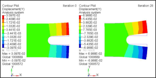
Create a third page.
1. From the menu bar, click Edit > Copy > Page.
2. From the menu bar, click Edit > Paste > Page.
Activate the first window and click to open the Contour panel.
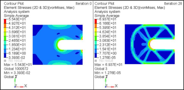
Under Result type, select Element Stresses (2D & 3D) (t).
Set Averaging method to Simple.
Click Apply.
In the first window, right-click and select Apply Style > Current Page > Contour from the context menu.

Figure 15.

Only use these stress results as a reference to help you understand how far from the limits the design is. Remember that topologic optimization will show you a concept shape. The stress results should be validated during the next design phases.