OS-T: 2095 Frequency Response Optimization of a Rectangular Plate
This tutorial demonstrates the capability of frequency response optimization using OptiStruct.
Initially, an existing finite element (FE) model of a flat plate is retrieved and modal frequency response analysis is performed to derive the peak magnitude. A dynamic response optimization is then performed on the same plate to obtain a new design.
- Objective
- Minimize volume.
- Constraints
- Max FRF Disp. < 600 mm
- Design Variables
- The density for each element in the design space.
Launch HyperMesh and Set the OptiStruct User Profile
-
Launch HyperMesh.
The User Profile dialog opens.
-
Select OptiStruct and click
OK.
This loads the user profile. It includes the appropriate template, macro menu, and import reader, paring down the functionality of HyperMesh to what is relevant for generating models for OptiStruct.
Import the Model
-
Click .
An Import tab is added to your tab menu.
- For the File type, select OptiStruct.
-
Select the Files icon
 .
A Select OptiStruct file browser opens.
.
A Select OptiStruct file browser opens. - Select the frf_response_input.fem file you saved to your working directory.
- Click Open.
- Click Import, then click Close to close the Import tab.
Apply Loads and Boundary Conditions
Create the SPC and Unit Load Collectors
-
Create the SPC load collector.
Figure 2. 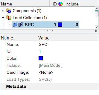
-
Create the unit-load collector.
Create Constraints
-
From the Model Browser, Load Collectors folder, right-click
on SPC and select Make Current
from the context menu.
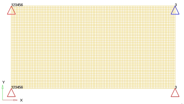
Figure 3. 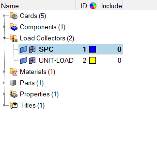
- From the Tool page, click numbers to open the numbers panel.
- Click from the extended entity selection menu.
- Enter the following numbers: 1, 2, 3, and 4.
- Click on.
- Click return.
- From the Analysis page, click the constraints panel.
- Confirm the create subpanel is selected using the radio buttons on the left-hand side of the panel.
-
Apply constraints to the nodes with IDs 1 and 2.
-
Apply a constraint to the node with ID 4.
- Using the nodes selector, select the node with ID 4.
- Uncheck all dofs, except dof3.
- Click create.
-
Create a unit load at a point on the flat plate.
- From the Model Browser, Load Collectors folder, right-click on unit-load and select Make Current from the context menu.
- In the Constraints panel, use the nodes selector to select the node with ID 3.
- Uncheck all dofs, except dof3.
- In the dof3= field, enter 20.
- Click load types= and select DAREA.
- Click create.
- Click return to go to the main menu.
Create a Frequency Range Curve
-
In the Model Browser, right-click and select .
The Curve Editor opens.
- For Name, enter tabled1.
-
In the table, enter:
- In the x(1) field, enter 0.0.
- In the y(1) field, enter 1.0.
- In the x(2) field, enter 1000.0.
- In the y(2) field, enter 1.0.
- Click the X in the upper right-hand corner to exit the dialog.
Figure 5. 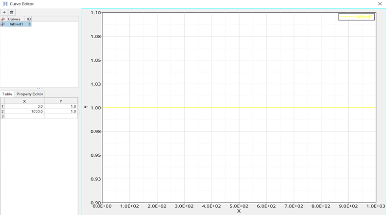
This provides a frequency range of 0.0 to 1000.0 with a constant load over this range.
- Click Color and select a color from the color palette.
- Set Card Image to TABLED1.
Create a Frequency Dependent Dynamic Load
- In the Model Browser, right-click and select .
- For Name, enter rload2.
- For Config type, select Dynamic Load - Frequency dependent.
- For Type, selectRLOAD2.
-
Define EXCITEID.
- Click .
- In the Select Loadcol dialog, select unit-load and click OK.
-
Define TB.
- Click Curves.
- In the Select Curves dialog, select tabled1 and click OK.
-
Set TYPE to LOAD.
This defines the input as a force.
Create a Set of Frequencies to be used in the Response Solution
-
In the Model Browser, right-click and select from the context menu.
A default load collector displays in the Entity Editor.
- For Name, enter freq5.
- Click Color and select a color from the color palette.
- Set Card Image to FREQi.
- Select FREQ5.
- In the NUMBER_OF_FREQ5= field, enter 1.
- In the FREQ5_MAX_NUMBER_OF_FR= field, enter 3.
-
Next to Data: ID, click
 .
.
-
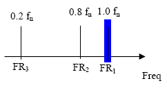
In the NUMBER OF FREQ = dialog, define frequencies values.
- In the F1 field, enter 1.0.
- In the F2 field, enter 1000.
- In the FR(0) field, enter 1.0.
- In the FR(1) field, enter 0.8.
- In the FR(2) field, enter 0.2.
- Click Close to exit the dialog.
Figure 6. 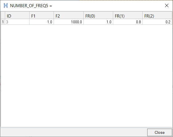
Create an EIGRL Load Step Input
Create EIGRL Load Step Input to use as the modal method.
- In the Model Browser, right-click and select
- For Name, enter eigrl.
- For Config Type, select Real Eigen Value Extraction .
- For Type, select EIGRL.
-
For ND, enter 17.
This specifies the eigenvalue extraction of the first 17 frequencies using the Lanczos method.
Create a Load Step
- From the Analysis page, click loadsteps.
- For Name, enter subcase1.
- Click type, and select Freq. resp (modal).
-
Define SPC.
- Check the box preceding SPC.
- Click the equal sign (=) and select spc from the load collector list.
-
Define METHOD (STRUCT).
- Check the box preceding METHOD (STRUCT).
- Click the equal sign (=) and select eigrl from the load step inputs list.
-
Define DLOAD.
- Check the box preceding DLOAD.
- Click the equal sign (=) and select rload2 from the load step inputs list.
-
Define FREQ.
- Check the box preceding FREQ.
- Click the equal sign (=) and select freq5 from the load collector list.
-
Click create.
Figure 8. 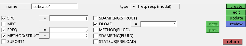
-
Click edit and define RESVEC.
- Select RESVEC.
- Set TYPE to APPLOAD.
- Set OPTION to YES.
An OptiStruct subcase has been created which references the constraints in the load collector, spc; the unit load in the load step input, rload2; with a set of frequencies defined in load collector, freq5 and modal method defined in the load step input, eigrl.
It is recommended to do a modal analysis before any FRF simulation. Here, this step is suppressed to focus on Frequency Response Analysis setup.
Create a Set of Nodes for Output of Results
-
In the Model Browser, right-click and select from the context menu.
A default set displays in the Entity Editor.
- For Name, enter SETA.
- Set Card Image to SET_GRID.
- Set Set Type to non-ordered.
- For Entity IDs, click .
-
Using the nodes selector, select the nodes with the ID of
3.
This is the node where the load was applied.
- In the panel area, click proceed.
- Click return to exit.
Create a Set of Outputs and Include Damping for Frequency Response Analysis
-
From the Analysis page, click the control cards
panel.
The Card Image dialog opens.
-
Define GLOBAL_OUTPUT_REQUEST.
-
Double-click SID(1) and select
SETA.
A value of 1 now appears below the SID field box. This sets the output for only the nodes in set 1.
Figure 9. 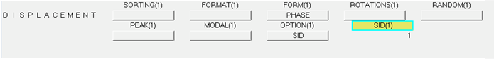
-
Double-click SID(1) and select
SETA.
-
Define FORMAT.
- Click FORMAT.
- In the number_of_formats= field, enter 2.
- Under FORMAT_V1, click the second instance of FORMAT and select OPTI.
- Click return.
-
Define PARAM.
-
Define OUTPUT.
- Click OUTPUT.
- Set KEYWORD to HGFREQ.
- Set FREQ to LAST.
- Leave number_of_outputs= set to 1.
- Click return.
- Click return to return to the main menu.
Save the Database
- From the menu bar, click .
- In the Save As dialog, enter frf_response_input.hm for the file name and save it to your working directory.
Submit the Job
-
From the Analysis page, click the OptiStruct
panel.
Figure 10. Accessing the OptiStruct Panel 
- Click save as.
-
In the Save As dialog, specify location to write the
OptiStruct model file and enter
frf_response_analysis for filename.
For OptiStruct input decks, .fem is the recommended extension.
-
Click Save.
The input file field displays the filename and location specified in the Save As dialog.
- Set the export options toggle to all.
- Set the run options toggle to analysis.
- Set the memory options toggle to memory default.
- Clear the options field.
- Click OptiStruct to launch the OptiStruct job.
View the Results
- In the OptiStruct panel, click HyperView to load the results from the analysis into the next page.
- From the menu bar, click .
-
In the Open Session File dialog, navigate to the directory
where the job was run and open the frf_response_analysis_freq.mvw file.
- Optional: If you launched from the OptiStruct panel, click Yes to discard the current session.
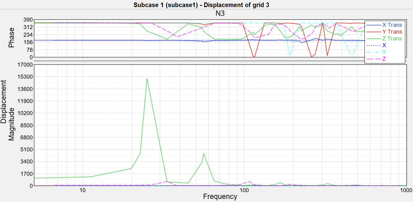
Two graphs are displayed. The graph title shows Subcase 1(subcase1)-Displacements of grid 3. The top graph shows Phase Angle verses Frequency. The bottom graph shows Displacement Response verses Frequency.Figure 11. 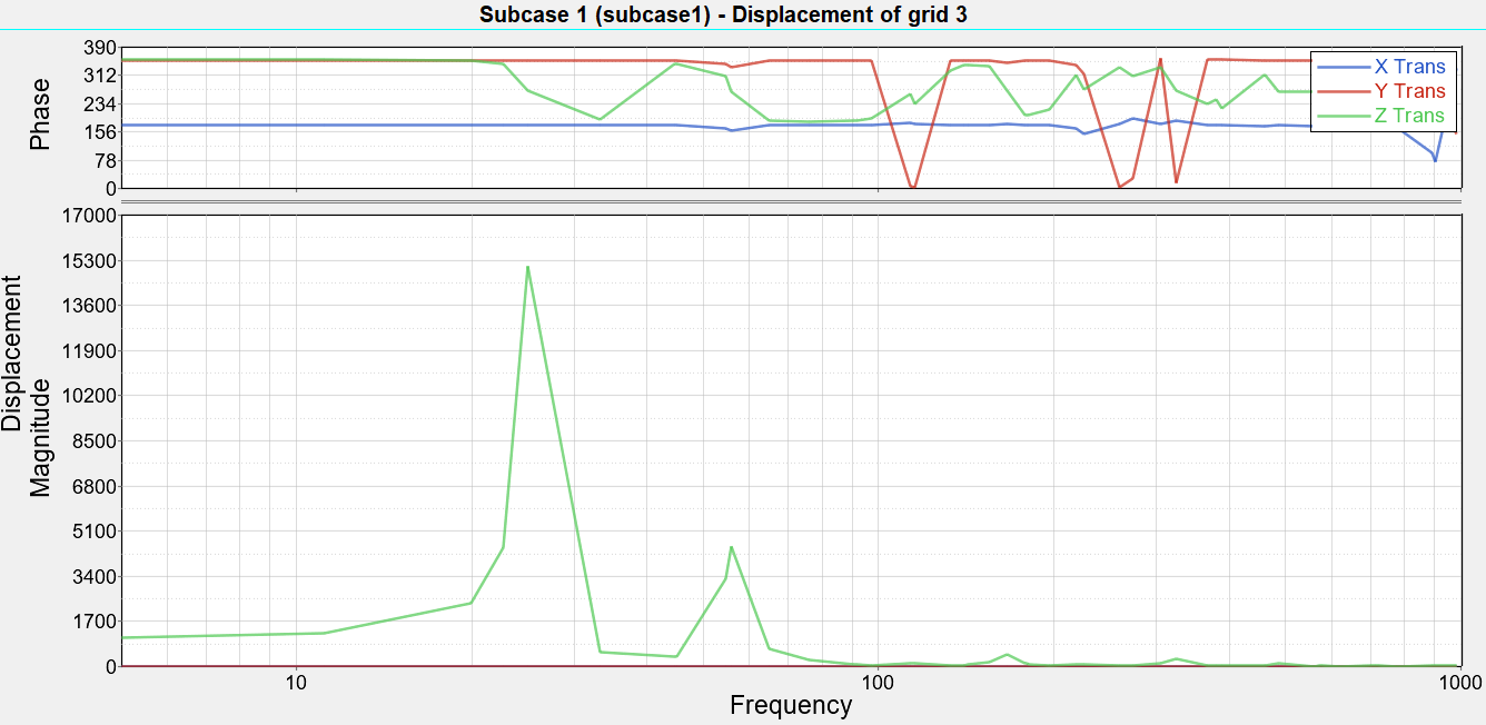
-
From the Curves toolbar, click
 to open the Define Curves panel.
-
Delete the X Trans and Y Trans curves.
The excitation is applied on Z direction then, the main effect will be detected on this direction.
-
On the Results toolbar, click
 to open the Curve Attributes panel.
-
Change the line attribute to continue
 .
.
-
Click the Symbol Attributes tab, and select the square
symbol.
Figure 12. 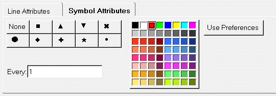
-
From the Annotations toolbar, click
 to open the Axes panel.
-
Change the Axis to Vertical.
Figure 13. 
- Click the Scale and Tics (Magnitude) tab, and select Logarithmic.
- In the Min field, enter 5.
- In the Max field, enter 200000.
- Click the Scale and Tics (Phase) tab, and change the Tics per axis to 7.
-
Set the Axis to Horizontal.
Figure 14. 
- In the Min field, enter 5.
-
In the Max field, enter 1000.
Figure 15. Frequency Response Function FRF (Node 3, Z-Displacement) 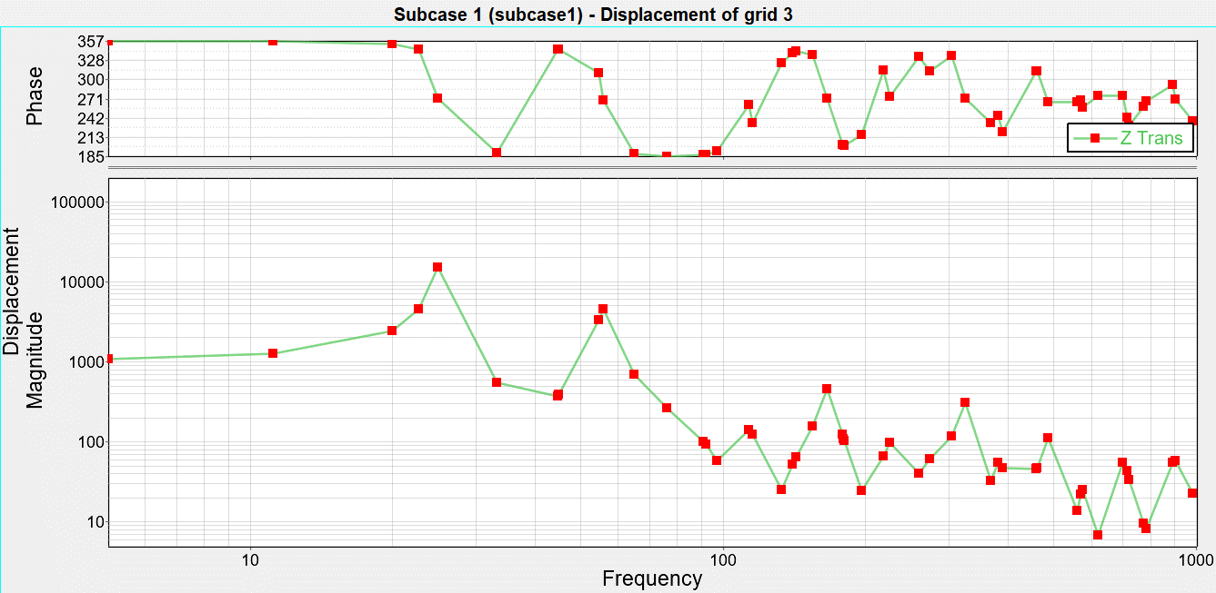
-
From the Curves toolbar, click
 to open the Coordinate Info panel.
-
Under Find point, select Magnitude.
Figure 16. 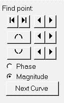
-
Click the maximum button to see the maximum Y-magnitude
~ 15055 in the table. The peak displacement of the baseline model.
Figure 17. 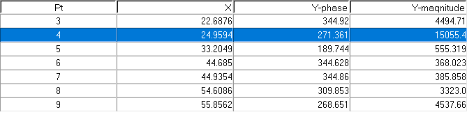
-
Return to HyperMesh by changing the client selector
to
 .
.
Open the Model
- Click .
- Select the frf_response_input.hm file you saved to your working directory.
-
Click Open.
The frf_response_input.hm database is loaded into the current HyperMesh session, replacing any existing data.
Save the Database
- From the menu bar, click .
- In the Save As dialog, enter frf_response_optimization.hm for the file name and save it to your working directory.
Set Up the Optimization
Create Topology Design Variables
- From the Analysis page, click optimization.
- Click topology.
- Select the create subpanel.
- In the desvar= field, enter plate.
- Set type: to PSHELL.
- Using the props selector, select Design.
- For base thickness, enter 0.15.
-
Click create.
A topology design space definition, shield, has been created. All elements referring to the design property collector (elements organized into the "design" component collector) are now included in the topology design space. The thickness of these shells can vary between 0.15 (base thickness) and the maximum thickness defined by the T (thickness) field on the PSHELL card.
The object of this exercise is to determine where to locate ribs in the designable region. Therefore, a non-zero base thickness is defined, which is the original thickness of the shells. The maximum thickness, which is defined by the T field on the PSHELL card, should be the allowable depth of the rib.
Currently, the T field on the PSHELL card is still set to 0.15 (the original shell thickness). You will change this to a higher value to create a design space where the material can be removed.
-
Update the design variable's parameters.
- Select the parameters subpanel.
- Toggle minmemb off to mindim=, then enter 2.0.
- Toggle maxmemb off to maxdim=, then enter 6.0.
- Click update.
- Click return.
-
Edit the thickness of the design property.
- In the Model Browser, Properties folder, click design.
- In the Entity Editor, T field, enter 1.000.
Create Optimization Responses
- From the Analysis page, click optimization.
- Click Responses.
-
Create the volume response, which defines the volume fraction of the design
space.
- In the responses= field, enter volume.
- Below response type, select volume.
- Set regional selection to total and no regionid.
- Click create.
-
Create the frequency response displacement (constraint), which defines the
maximum magnitude on dof3.
- In the responses= field, enter frfdisp.
- Set the response type to frf displacement.
- Switch the component from real to magnitude.
- Set the function to all freq.
- Using the nodes selector, select the node with ID 3.
- Select dof3.
- Click create.
- Click return to go back to the Optimization panel.
Create Design Constraints
- Click the dconstraints panel.
- In the constraint= field, enter constr.
- Click response = and select frfdisp.
- Check the box next to upper bound, then enter 600.
- Using the loadsteps selector, select subcase1.
- Click create.
- Click return to go back to the Optimization panel.
Define the Objective Function
- Click the objective panel.
- Verify that min is selected.
- Click response= and select volume.
- Click create.
- Click return twice to exit the Optimization panel.
Run the Optimization
- From the Analysis page, click OptiStruct.
- Click save as.
-
In the Save As dialog, specify location to write the
OptiStruct model file and enter
frf_response_optimization for filename.
For OptiStruct input decks, .fem is the recommended extension.
-
Click Save.
The input file field displays the filename and location specified in the Save As dialog.
- Set the export options toggle to all.
- Set the run options toggle to optimization.
- Set the memory options toggle to memory default.
-
Click OptiStruct to run the optimization.
The following message appears in the window at the completion of the job:
OPTIMIZATION HAS CONVERGED.
FEASIBLE DESIGN (ALL CONSTRAINTS SATISFIED).
OptiStruct also reports error messages if any exist. The file frf_response_optimization.out can be opened in a text editor to find details regarding any errors. This file is written to the same directory as the .fem file. - Click Close.
- frf_response_optimization.hgdata
- HyperGraph file containing data for the objective function, percent constraint violations, and constraint for each iteration.
- frf_response_optimization.HM.comp.tcl
- HyperMesh command file used to organize elements into components based on their density result values. This file is only used with OptiStruct topology optimization runs.
- frf_response_optimization.HM.ent.tcl
- HyperMesh command file used to organize elements into entity sets based on their density result values. This file is only used with OptiStruct topology optimization runs.
- frf_response_optimization.html
- HTML report of the optimization, giving a summary of the problem formulation and the results from the final iteration.
- frf_response_optimization.oss
- OSSmooth file with a default density threshold of 0.3. You may edit the parameters in the file to obtain the desired results.
- frf_response_optimization.out
- OptiStruct output file containing specific information on the file setup, the setup of the optimization problem, estimates for the amount of RAM and disk space required for the run, information for all optimization iterations, and compute time information. Review this file for warnings and errors that are flagged from processing the frf_response_optimization.fem file.
- frf_response_optimization.sh
- Shape file for the final iteration. It contains the material density, void size parameters and void orientation angle for each element in the analysis. This file may be used to restart a run.
- frf_response_optimization.stat
- Contains information about the CPU time used for the complete run and also the break-up of the CPU time for reading the input deck, assembly, analysis, convergence, and so on.
- frf_response_optimization_des.h3d
- HyperView binary results file that contain optimization results.
- frf_response_optimization_s#.h3d
- HyperView binary results file that contains from linear static analysis, and so on.
- frf_response_optimization.his_data
- The OptiStruct history file containing iteration number, objective function values and percent of constraint violation for each iteration.
View the Results
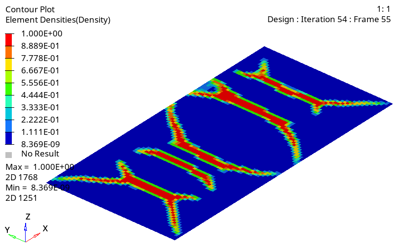
Element Density and Element Thickness results are output from OptiStruct for all iterations.
View a Static Plot of the Density Results
- From the OptiStruct panel, click HyperView.
-
Open the frf_response_optimization.mvw
session file.
- From the menu bar, click .
- In the Open Session File dialog, navigate to your working directory and open the frf_response_optimization.mvw session file.
-
From the Results toolbar, click
 to open the Contour panel.
-
In the Results Browser, select the last
load case simulation.
Figure 18. 
- In the Contour panel, set the averaging method to simple.
- Click apply.
Compare the Peak Displacement of the Optimization Run
-
Open the FRF_response_analysis_freq.mvw
session file.
- From the menu bar, click .
- In the Open Session File dialog, navigate to your working directory and open the FRF_response_analysis_freq.mvw session file.
-
On the Curves toolbar, click
 to open the Build Plots panel,
which you will use to add curves on top of the existing
analysis information.
to open the Build Plots panel,
which you will use to add curves on top of the existing
analysis information.
-
In the Data file field, load the frf_response_optimization_s2.h3d
optimization file, which contains the final iteration
analysis.
Figure 20. 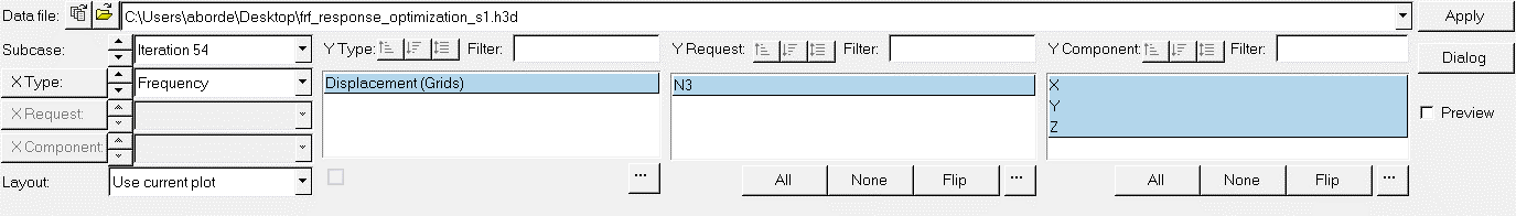
- Set Subcase to the last iteration.
- Set X Type to Frequency.
- For Y Type, select Displacement (Grids).
- For Y Request, select N3.
- For Y Component, select X, Y, and Z.
- Click Apply to overlay the new information onto the original plot.