
OS-T: 4070 Free-sizing Nonlinear Gap Optimization on an Airplane Wing Rib
In this tutorial you will use an existing finite element model of an aluminum wing rib model to demonstrate how to do free-sizing optimization.
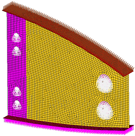
There are four shell components in the model: the mounting flange, the web, the top and bottom flanges, and the lug. The web is connected to the lug by gap elements. Appropriate properties, loads, boundary conditions, and nonlinear subcases have already been defined in the model. The design region is the web and the rest of the components are non-design. Since a large portion of aerospace components are shell structures which are manufactured by machining or milling operations, free-sizing optimization is very suitable for those components. To understand the limitations of topology optimization for such applications, a nonlinear gap topology optimization will also be done on the wing rib model.
- Objective
- Minimize weighted compliance WCOMP.
- Constraints
- Volume fraction on the web < 0.3.
- Design Variables for Free Sizing Optimization
- Thickness of each shell element in the design space.
- Design Variables for Topology Optimization
- Element density of each element in the design domain.
Launch HyperMesh and Set the OptiStruct User Profile
The model being used for this exercise is that of a control arm (Figure 6). Loads and boundary conditions and two static loadcases have already been defined on this model.
The model being used for this exercise is that of an automotive frame (OS-T: 6030 Seam Weld Fatigue using S-N MethodOS-T: 6040 Spot Weld Fatigue using S-N MethodFigure 1). The input file consists of 3 static loadsteps to which the frame is subjected to – Frontal torsion, Rear torsion and the Vertical bending.
The model being used for this exercise is that of a simple CAD box (Figure 1). Four loadsteps have already been defined on this model, each of which represent Normal Modes Analysis, Frequency Response at both the constraint points and the Random Response Analysis.
The model being used for this exercise is that of bracket_frf_EN (Figure 1). Three loadsteps have already been defined on this model, each of which represent Static Analysis, Normal Modes Analysis and Frequency Response excited at the loading point.
-
Launch HyperMesh.
The User Profile dialog opens.
-
Select OptiStruct and click
OK.
This loads the user profile. It includes the appropriate template, macro menu, and import reader, paring down the functionality of HyperMesh to what is relevant for generating models for OptiStruct.
- Click .
- For New Session, enter a name in your working directory folder.
-
Click Create.
This creates a new file to save the instance of the currently loaded fatigue process template.
Perform a Free-Sizing Nonlinear Gap Optimization
Open the Model
- Click .
- Select the rib_complete.hm file you saved to your working directory.
-
Click Open.
The rib_complete.hm database is loaded into the current HyperMesh session, replacing any existing data.
Set Up the Optimization
Create Free-sizing Optimization Design Variables
- From the Analysis page, click the optimization panel.
- Click the free size panel.
- Select the create subpanel.
- In the desvar= field, enter shells.
- Set type to PSHELL.
- Using the props selector, select the Web component.
- Click create.
Create Free-sizing Manufacturing Constraints
- Select the parameters subpanel.
- Click desvars and select shells.
- Toggle minmemb off to mindim =, and enter 2.0.
- Click update.
- Click return.
Create Optimization Responses
- From the Analysis page, click optimization.
- Click Responses.
-
Create the volume fraction response.
- In the responses= field, enter Volfrac.
- Below response type, select volumefrac.
- Set regional selection to total and no regionid.
- Click create.
-
Create the weighted component response.
- In the responses= field, enter wcomp.
- Below response type, select weighted comp.
- Click loadsteps, then select all loadsteps.
- Click return.
- Click create.
- Click return to go back to the Optimization panel.
Create Design Constraints
- Click the dconstraints panel.
- In the constraint= field, enter vol.
- Click response = and select volfrac.
- Check the box next to upper bound, then enter 0.3.
- Click create.
- Click return to go back to the Optimization panel.
Define the Objective Function
- Click the objective panel.
- Verify that min is selected.
- Click response= and select wcomp.
- Click create.
- Click return twice to exit the Optimization panel.
Run the Optimization
- From the Analysis page, click OptiStruct.
- Click save as.
-
In the Save As dialog, specify location to write the
OptiStruct model file and enter
rib_freesize for filename.
For OptiStruct input decks, .fem is the recommended extension.
-
Click Save.
The input file field displays the filename and location specified in the Save As dialog.
- Set the export options toggle to all.
- Set the run options toggle to optimization.
- Set the memory options toggle to memory default.
-
Click OptiStruct to run the optimization.
The following message appears in the window at the completion of the job:
OPTIMIZATION HAS CONVERGED.
FEASIBLE DESIGN (ALL CONSTRAINTS SATISFIED).
OptiStruct also reports error messages if any exist. The file rib_freesize.out can be opened in a text editor to find details regarding any errors. This file is written to the same directory as the .fem file. - Click Close.
- rib_freesize.hgdata
- HyperGraph file containing data for the objective function, percent constraint violations, and constraint for each iteration.
- rib_freesize.hist
- The OptiStruct iteration history file containing the iteration history of the objective function and of the most violated constraint. Can be used for a xy plot of the iteration history.
- rib_freesize.HM.comp.tcl
- HyperMesh command file used to organize elements into components based on their density result values. This file is only used with OptiStruct topology optimization runs.
- rib_freesize.HM.ent.tcl
- HyperMesh command file used to organize elements into entity sets based on their density result values. This file is only used with OptiStruct topology optimization runs.
- rib_freesize.html
- HTML report of the optimization, giving a summary of the problem formulation and the results from the final iteration.
- rib_freesize.mvw
- HyperView session file.
- rib_freesize.oss
- OSSmooth file with a default density threshold of 0.3. You may edit the parameters in the file to obtain the desired results.
- rib_freesize.out
- OptiStruct output file containing specific information on the file setup, the setup of the optimization problem, estimates for the amount of RAM and disk space required for the run, information for all optimization iterations, and compute time information. Review this file for warnings and errors that are flagged from processing the rib_freesize.fem file.
- rib_freesize.res
- HyperMesh binary results file.
- rib_freesize.sh
- Shape file for the final iteration. It contains the material density, void size parameters and void orientation angle for each element in the analysis. This file may be used to restart a run.
- rib_freesize.stat
- Contains information about the CPU time used for the complete run and also the break-up of the CPU time for reading the input deck, assembly, analysis, convergence, and so on.
- rib_freesize_des.h3d
- HyperView binary results file that contain optimization results.
- rib_freesize_frame.html
- HTML file used to post-process the .h3d with HyperView Player using a browser. It is linked with the _menu.html file.
- rib_freesize_hist.mvw
- Contains the iteration history of the objective, constraints, and the design variables. It can be used to plot curves in HyperGraph, HyperView, and MotionView.
- rib_freesize_menu.html
- HTML file used to post-process the .h3d with HyperView Player using a browser.
- rib_freesize_s#.h3d
- HyperView binary results file that contains from linear static analysis, and so on.
- rib_freesize.fsthick
- The element definitions for those elements that were part of a free size design space. The optimized thickness of these elements is provided as nodal thickness values (Ti).
View the Results
-
From the OptiStruct panel, click HyperView.
HyperView launches within the HyperMesh Desktop and the results from the rib_freesize.h3d file are loaded.
-
On the Visualization toolbar, click
 to open the Entity Attributes panel..
-
Select Auto appy mode: Display Off, then select the
Web component.
All of the components are undisplayed except Web.
-
Click the Mesh shaded mesh option
 .
.
- Click the Web component to get a shaded mesh.
-
On the Results toolbar, click
 to open the Contour panel.
- Set the Result type to Element Thicknesses.
-
In the Results Browser, select the last iteration listed in
the Simulation list.
Figure 2. 
-
On the Standard Views toolbar, click
 to show the top view of the Web.
The contour element thickness on the Web component displays.
The result from free-sizing optimization is a web with optimized thickness distribution that can be reduced subsequently into larger zones for simplification of the manufacturing process. Moreover, the design obtained from free-sizing offers the freedom to create cavities, ribs, and varying thickness simultaneously, which is not possible in topology optimization.Figure 3. Thickness contour from free-sizing nonlinear gap optimization. on the Web of plate thickness 0.1mm 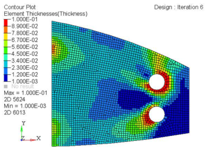
-
On the Page Controls toolbar, click
 to close the HyperView client pages until the
HyperMesh client displays.
to close the HyperView client pages until the
HyperMesh client displays.
Save the Database
- From the menu bar, click .
- In the Save As dialog, enter rib_complete.hm for the file name and save it to your working directory.
Perform a Topology Nonlinear Gap Optimization
Set Up a Topology Optimization with Nonlinear Gap Elements
Create Topology Design Variables
- In the Model Browser, right-click on the Design Variable folder and select Delete from the context menu.
- From the Analysis page, click the optimization panel.
- Click the topology panel.
- Select the create subpanel.
- In the desvar = field, enter shells.
- Using the props selector, select the Web component.
- Set type to PSHELL.
- Leave the base thickness as 0.0.
- Click create.
Save the Database
- From the menu bar, click .
- In the Save As dialog, enter rib_topology.hm for the file name and save it to your working directory.
Create Topology Optimization Manufacturing Constraints
- Select the parameters subpanel.
- Click desvars = and select shells.
- Toggle minmemb off to mindim =, then enter 2.0 for minimum member size control.
- Click update.
- Click return twice.
Run the Optimization
- From the Analysis page, click OptiStruct.
- Click save as.
-
In the Save As dialog, specify location to write the
OptiStruct model file and enter
rib_topology for filename.
For OptiStruct input decks, .fem is the recommended extension.
-
Click Save.
The input file field displays the filename and location specified in the Save As dialog.
- Set the export options toggle to all.
- Set the run options toggle to optimization.
- Set the memory options toggle to memory default.
-
Click OptiStruct to run the optimization.
The following message appears in the window at the completion of the job:
OPTIMIZATION HAS CONVERGED.
FEASIBLE DESIGN (ALL CONSTRAINTS SATISFIED).
OptiStruct also reports error messages if any exist. The file rib_topology.out can be opened in a text editor to find details regarding any errors. This file is written to the same directory as the .fem file. - Click Close.
View the Results
-
From the OptiStruct panel, click HyperView.
HyperView launches within the HyperMesh Desktop and the results from the rib_topology.mvw file are loaded. This file is linked with the .h3d file where the model and results are defined.
-
On the Visualization toolbar, click to open the Entity Attributes panel.
-
Select Auto appy mode: Display Off, then select the
Web component.
All of the components are undisplayed except Web.
-
Click the Mesh shaded mesh option .
- Click the Web component to get a shaded mesh.
-
On the Results toolbar, click to open the Contour panel.
- Set the Result type to Element Densities.
- In the Results Browser, select the last iteration listed in the Simulation list.
-
On the Standard Views toolbar, click to show the top view of the Web.
- Click Apply to show the contour of element density on the Web component.
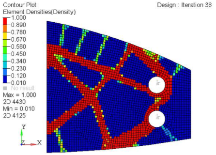
Review and Compare Results from Free-size Optimization and Topology Optimization
Results from the topology optimization show a truss type design with extensive cavities and voids, while the results from free-sizing optimization tend to come up with shear panels. While solid/void density distribution is the only choice for solid elements; for shell structures, intermediate densities can be interpreted as different thicknesses and penalizing then could result in potentially inefficient shell structures. Moreover, since a large portion of aerospace structures are shell structures, a shear panel type design is often desirable for manufacturing purposes especially for machine milled shell structures. Free-sizing optimization can prove to be very beneficial in those situations.