In this tutorial you will perform a size optimization for a model comprised of shell
and bar elements. You will update the PBARL property to simulate the
properties of the bar elements and then link that to the design variable. The resulting
design will have higher frequencies and updated element properties.
Before you begin, copy the file(s) used in this tutorial to your
working directory.
Size optimizations involve the changing of the properties of either 1D or 2D
elements. These properties include area, moments of inertia of the 1D elements, and
the thickness of 2D elements. Size optimization is performed when it is not
necessary to remove materials, generate beads or change the shape of the
structure.
With size optimization, the cross-sectional properties of the elements are changed to
meet the necessary objective. Properties are linked with design variables
(DESVAR) using DVPREL cards.
This tutorial outlines using OptiStruct macros under an
OptiStruct user profile to setup the optimization
problem.Figure 1. Finite Element Model of a Shredder
The optimization problem is stated as:
Objective
Minimize the global mass.
Constraints
Transverse modes higher than 6 Hz.
Design Variables
Beam width, beam thickness, beam depth, and shell thickness.
Launch HyperMesh and Set the OptiStruct User Profile
Launch HyperMesh.
The User Profile dialog opens.
Select OptiStruct and click
OK.
This loads the user profile. It includes the appropriate template, macro
menu, and import reader, paring down the functionality of HyperMesh to what is relevant for generating models for
OptiStruct.
Import the Model
Click File > Import > Solver Deck.
An Import tab is added to your tab menu.
For the File type, select OptiStruct.
Select the Files icon .
A Select OptiStruct file browser
opens.
Select the shredder.fem file you saved
to your working directory.
Click Open.
Click Import, then click Close to
close the Import tab.
Perform Finite Element Analysis and Check Results
Submit the Job
From the Analysis page, click the OptiStruct
panel.
Figure 2. Accessing the OptiStruct Panel
Click save as.
In the Save As dialog, specify location to write the
OptiStruct model file and enter
shredder_analysis for filename.
For OptiStruct input decks,
.fem is the recommended extension.
Click Save.
The input file field displays the filename and location specified in the
Save As dialog.
Set the export options toggle to all.
Set the run options toggle to analysis.
Set the memory options toggle to memory default.
Click OptiStruct to launch
the OptiStruct job.
If the job is successful, new results files
should be in the directory where the shredder_analysis.fem was written. The shredder_analysis.out file is a good place to look for error messages that could help
debug the input deck if any errors are present.
View the Eigen Modes
From the OptiStruct panel, click HyperView.
HyperView launches within the HyperMesh Desktop and a new page
and session file, shredder_analysis.mvw, loads. This file is linked with
the shredder_analysis.h3d
file, which contains the model and results.
On the Animation toolbar, set the animation type to (Modal).
On the Results toolbar, click to open the Deformed
panel.
Define deformed shape settings.
Set the Result type to Eigen
Mode(v).
Set Scale to Model
Units.
Set Type to
Uniform.
In the Value field, enter
1000.
This means that the maximum displacement will be 1000
modal units and all other displacements will be
proportional.
Using a scale factor higher than 1.0, amplifies the
deformations while a scale factor smaller than 1.0
would reduce them. In this case, you are
accentuating displacements in all directions.
Define undefomed shape settings.
Set Show to Edges.
Set Color to Mesh.
Click Apply.
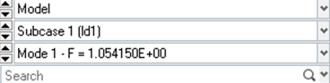
In the Results Browser, from the list of
simulations, select Mode 1.
Figure 3.
On the Results toolbar, click to open the Contour panel.
Click Apply.
The Eigen Mode contour is plotted.
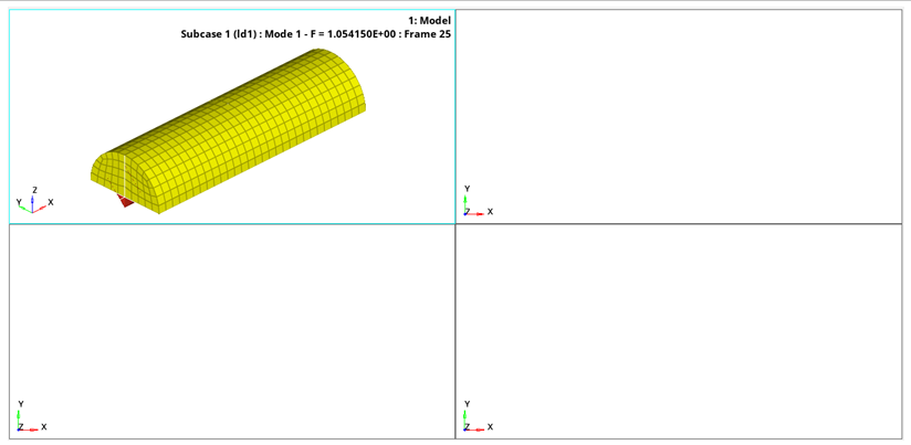
On the Page Controls toolbar, set the page layout to .
Figure 4.
Click the first window, then click Edit > Copy > Window from the menu bar.
Click the second window, then click Edit > Paste > Window from the menu bar.
Copy the first window into the third and fourth windows.
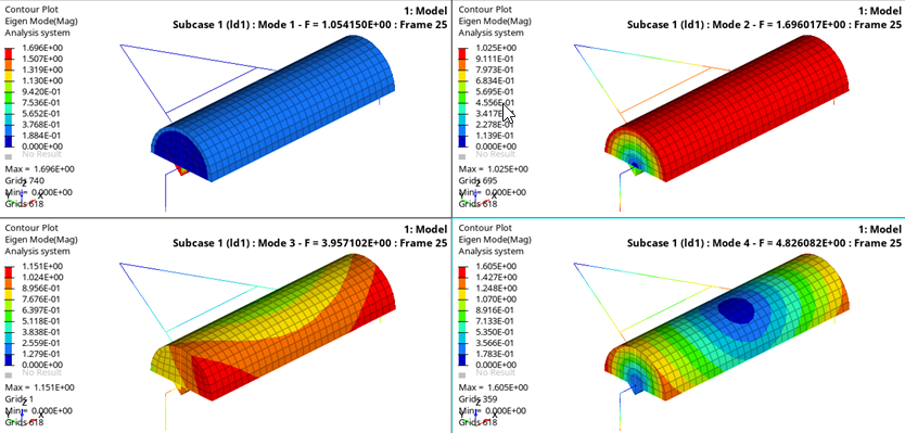
Figure 5. Contour of First Mode on all Windows
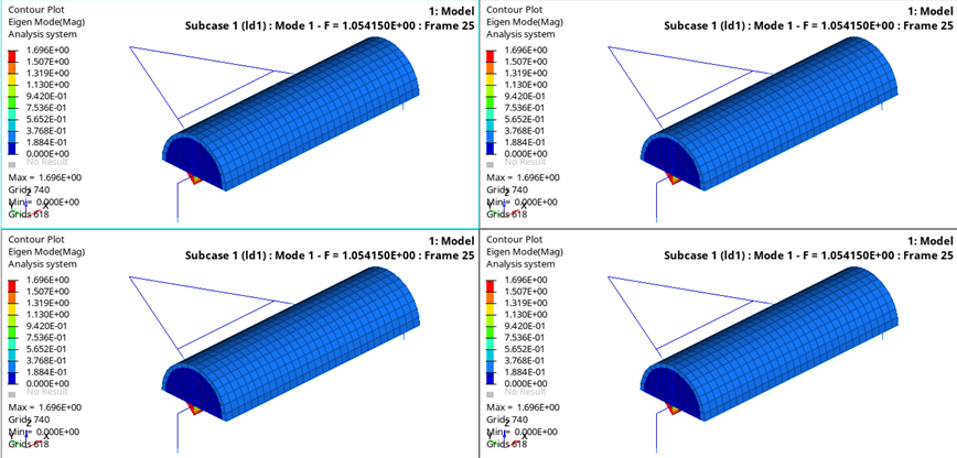
Change the mode assigned to the windows by clicking a window to
make it active, then selecting a mode in the Results Browser.
Set the second window to Mode 2.
Set the third window to Mode 3.
Set the fourth window to Mode 4.
Figure 6.
Figure 7. Contour Plot for the First Four Eigen Modes
On the Animation toolbar, click to start the animation. Click
again to stop the animation.
The third and fourth mode (~ 3.9 and 4.8 Hz) has a transversal
shape that can reduce the performance of the shredder when
it gets excited. The objective, then, is to get the minimum
mass to greater than 7Hz.
From the menu bar, click File > Save As > Report Template.
In the Save Report As dialog, navigate to
your working directory and save the file as
report.tpl.
Figure 8.
In the top, right of the application, click and
to navigate
back to the HyperMesh client on
the first page.
Set Up the Optimization
Define Design Variables
The design variables for this problem are the thickness of the cover, width, thickness, and
depth of the bar. You will define the first design variable using the Size
panel.
From the Analysis page, click the optimization
panel.
Click the size panel.
Select the desvar subpanel.
Create the design variable, coverthck.
In the desvar = field, enter coverthck.
In the initial value = field, enter 3.0.
In the lower bound = field, enter 1.0.
In the upper bound = field, enter 6.0.
Set the move limit toggle to move limit
default.
Set the discrete design variable (ddval) toggle to no
ddval.
Click create.
Create four more design variables.
Design Variable
Initial Value
Lower Bound
Upper Bound
Beamwide
50
30
90
Beamhigh
100
80
125
Beamthck1
10
5
15
Beamthck2
20
15
30
Select the generic relationship subpanel.
Create a design variable property relationship, coverthck.
In the name = field, enter coverthck.
In the C0 field, enter 0.0.
Using the prop selector, select cover.
Under the props selector, select Thickness
T.
Click designvars, select
coverthck, and click
return.
Click create.
In the next steps you will define property relations for beam dimensions.
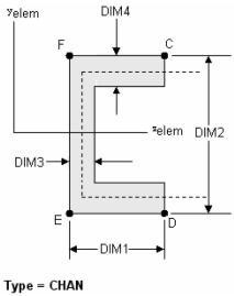
Each dimension of a C beam will be defined as a design variable.Figure 9.
Table 1. Property Values on the Initial Design
Name
Represents
Value
DIMs(1)
Beam Width
50
DIMs(2)
Beam High
100
DIMs(3)
Beam Thck1
10
DIMs(4)
Beam Thck2
20
Create a design variable property relationship, DIM1.
In the name = field, enter DIM1.
In the C0 field, enter 0.0.
Using the prop selector, select frame2.
Under the props selector, select Dimension
1.
Click designvars, select
Beamwide, and click
return.
Click create.
Create a design variable property relationship, DIM2.
In the name = field, enter DIM2.
In the C0 field, enter 0.0.
Using the prop selector, select frame2.
Under the props selector, select Dimension
2.
Click designvars, select
Beamhigh, and click
return.
Click create.
Create a design variable property relationship, DIM3.
In the name = field, enter DIM3.
In the C0 field, enter 0.0.
Using the prop selector, select frame2.
Under the props selector, select Dimension
3.
Click designvars, select
Beamthck1, and click
return.
Click create.
Create a design variable property relationship, DIM4.
In the name = field, enter DIM4.
In the C0 field, enter 0.0.
Using the prop selector, select frame2.
Under the props selector, select Dimension
4.
Click designvars, select
Beamthck2, and click
return.
Click create.
Click return to go back to the Optimization panel.
Create Optimization Responses
From the Analysis page, click optimization.
Click Responses.
Create the mass response, which is defined for the total volume of the
model.
In the responses= field, enter mass.
Below response type, select mass.
Set regional selection to total and
no regionid.
Click create.
Create the frequency response.
In the responses= field, enter f3.
Below response type, select frequency.
For Mode Number, enter 3.
Click create.
A response, f3, is defined for
the frequency of the third mode
extracted.
Create another frequency response, named f4, for mode 4.
Click return to go back to the Optimization panel.
Define Constraints
Click the dconstraints panel.
Create the constraint, c_f3.
In the constraint= field, enter c_f3.
Check the box next to lower bound, then enter
6.0.
Click response = and select
f3.
Using the loadsteps selector, select ld1.
Click create.
Create the constraint, c_f4.
In the constraint= field, enter c_f4.
Check the box next to lower bound, then enter
6.0.
Click response = and select
f4.
Using the loadsteps selector, select ld1.
Click create.
Click return to exit the panel.
Define the Objective Function
Click the objective panel.
Verify that min is selected.
Click response and select mass.
Click create.
Click return twice to exit the Optimization panel.
Save the Database
From the menu bar, click File > Save As > Model.
In the Save As dialog, enter shredder_optimization.hm for the file name and save it to your
working directory.
Run the Optimization
From the Analysis page, click OptiStruct.
Click save as.
In the Save As dialog, specify location to write the
OptiStruct model file and enter
shredder_optimization for filename.
For OptiStruct input decks,
.fem is the recommended extension.
Click Save.
The input file field displays the filename and location specified in the
Save As dialog.
Set the export options toggle to all.
Set the run options toggle to optimization.
Set the memory options toggle to memory default.
Click OptiStruct to run the optimization.
The following message appears in the window at the completion of the
job:
OPTIMIZATION HAS CONVERGED.
FEASIBLE DESIGN (ALL CONSTRAINTS SATISFIED).
OptiStruct also reports error messages if any exist. The
file shredder_optimization.out can be opened in a
text editor to find details regarding any errors. This file is written to the
same directory as the .fem file.
Click Close.
View the Results
From the OptiStruct panel, click HyperView.
HyperView launches within the HyperMesh Desktop and the results are
loaded.
In the top, right of the application, click
and
to navigate to the Design History page.
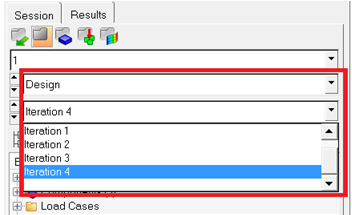
In the Results Browser, select the last iteration.
Figure 10.
On the Results toolbar, click
to open the Contour panel.
Set the Result type to Element Thicknesses (s) and
Thickness.
Click Apply.
The resulting colors represent the thickness fields resulting from the
applied loads and boundary conditions. The final optimized thickness of the
cover component is 1.0.
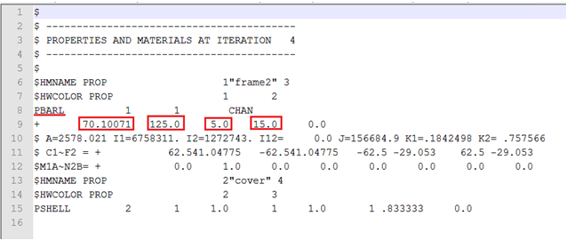
Open the shredder_optimization.prop file using any
text editor to review final optimized PBAR property.
Figure 11. The final dimensions could be rounded off to:
Beam Wide (DIM1)
70.10
Beam High (DIM2)
125
Beam Thck (DIM3)
5
Beam wide (DIM4)
15
This .prop file can be read into HyperMesh with over write mode on and the
PBARL card will be updated.

 .
A Select OptiStruct file browser opens.
.
A Select OptiStruct file browser opens.
 (Modal).
 to open the Deformed
panel.
to open the Deformed
panel.
 to open the Contour panel.
 .
.
 to start the animation. Click
again to stop the animation.
The third and fourth mode (~ 3.9 and 4.8 Hz) has a transversal shape that can reduce the performance of the shredder when it gets excited. The objective, then, is to get the minimum mass to greater than 7Hz.
to start the animation. Click
again to stop the animation.
The third and fourth mode (~ 3.9 and 4.8 Hz) has a transversal shape that can reduce the performance of the shredder when it gets excited. The objective, then, is to get the minimum mass to greater than 7Hz.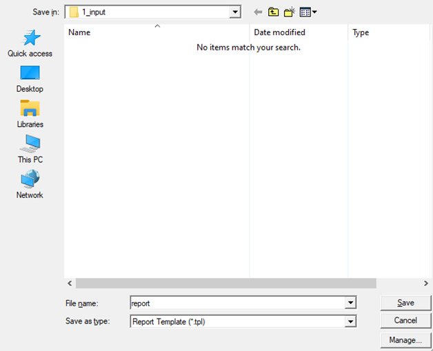
 and
and
 to navigate
back to the HyperMesh client on
the first page.
to navigate
back to the HyperMesh client on
the first page.