
OS-T: 4000 3D Size Optimization of a Rail Joint
In this tutorial you will perform a size optimization on an automobile rail joint modeled with shell elements.
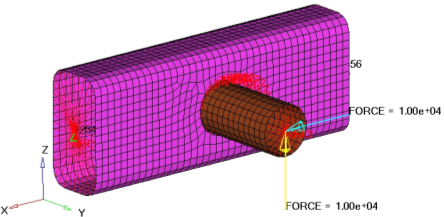
You will load the structural model into HyperMesh. The constraints, loads, material properties, and subcases (loadsteps) are already defined in the model. Size design variables and optimization parameters are defined, and OptiStruct determines the optimal gauges for the components. The results are then reviewed in HyperView.
- Objective
- Minimize volume.
- Constraints
- A given maximum nodal displacement at the loading grid point for two loading conditions.
- Design Variables
- Gauges of the two parts.
Launch HyperMesh and Set the OptiStruct User Profile
-
Launch HyperMesh.
The User Profile dialog opens.
-
Select OptiStruct and click
OK.
This loads the user profile. It includes the appropriate template, macro menu, and import reader, paring down the functionality of HyperMesh to what is relevant for generating models for OptiStruct.
Open the Model
- Click .
- Select the joint_size.hm file you saved to your working directory.
-
Click Open.
The joint_size.hm database is loaded into the current HyperMesh session, replacing any existing data.
Set Up the Optimization
Create Size Design Variables
- From the Analysis page, click the optimization panel.
- Click the size panel.
- Select the desvar subpanel.
-
Create the design variable, tube.
- In the desvar = field, enter tube.
- In the initial value = field, enter 1.0.
- In the lower bound = field, enter 0.1.
- In the upper bound = field, enter 5.0.
- Set the move limit toggle to move limit default.
- Set the discrete design variable (ddval) toggle to no ddval.
- Click create.
-
Create the design variable, rail.
- In the desvar = field, enter rail.
- In the initial value = field, enter 1.0.
- In the lower bound = field, enter 0.1.
- In the upper bound = field, enter 5.0.
- Set the move limit toggle to move limit default.
- Set the discrete design variable (ddval) toggle to no ddval.
- Click create.
- Select the generic relationship subpanel.
-
Create a design variable property relationship, tube_th.
A design variable property relationship, tube_th, has been created relating the design variable tube to the thickness entry on the PSHELL card for the property tube2.
-
Create a design variable property relationship, rail_th.
- In the name = field, enter rail_th.
- Using the prop selector, select tube1.
- Under the props selector, select Thickness T.
- Click designvars.
- Select rail.
- Click return.
- Click create.
A design variable property relationship, rail_th, has been created relating the design variable rail to the thickness entry on the PSHELL card for the property tube1. - Click return to go to the Optimization panel.
Create Responses
- Click the responses panel.
-
Create the response, volume.
- In the response= field, enter volume.
- Set the response type to volume.
- Set the regional selection to total.
- Click create.
The response, volume, is defined for the total volume of the model. -
Create the response, X_Disp.
The response, X_Disp, is defined for the x-displacement of the node 3143.
-
Create the response, Z_Disp.
The response, Z_Disp, is defined for the z-displacement of the node 3143.
- Click return to go to the Optimization panel.
Create Constraints
A response defined as the objective cannot be constrained. In this case, you cannot constrain the response volume.
Upper bound constraints are to be defined for the responses X_Disp and Z_Disp.
- Click the dconstraints subpanel.
-
Define a constraint on the response X_Disp.
- In the constraints= field, enter Disp_X.
- Check the box next to upper bound, then enter 0.9.
- Click response = and select X_Disp.
- Using the loadsteps selector, select Force_X.
- Click create.
The constraint is an upper bound with a value of 0.9. The constraint applies to the subcase Force_X. -
Define a constraint on the response Z_Disp.
- In the constraints= field, enter Disp_Z.
- Check the box next to upper bound, then enter 1.6.
- Click response = and select Z_Disp.
- Using the loadsteps selector, select Force_Z.
- Click create.
The constraint is an upper bound with a value of 1.6. The constraint applies to the subcase Force_Z. - Click return to go to the Optimization panel.
Define the Objective Function
- Click the objective panel.
- Verify that min is selected.
- Click response and select volume.
- Click create.
- Click return twice to exit the Optimization panel.
Save the Database
- From the menu bar, click .
- In the Save As dialog, enter joint_sizeOPT.hm for the file name and save it to your working directory.
Run the Optimization
- From the Analysis page, click OptiStruct.
- Click save as.
-
In the Save As dialog, specify location to write the
OptiStruct model file and enter
joint_sizeOPT for filename.
For OptiStruct input decks, .fem is the recommended extension.
-
Click Save.
The input file field displays the filename and location specified in the Save As dialog.
- Set the export options toggle to all.
- Set the run options toggle to optimization.
- Set the memory options toggle to memory default.
-
Click OptiStruct to run the optimization.
The following message appears in the window at the completion of the job:
OPTIMIZATION HAS CONVERGED.
FEASIBLE DESIGN (ALL CONSTRAINTS SATISFIED).
OptiStruct also reports error messages if any exist. The file joint_sizeOPT.out can be opened in a text editor to find details regarding any errors. This file is written to the same directory as the .fem file. - Click Close.
- joint_sizeOPT.hgdata
- HyperGraph file containing data for the objective function, percent constraint violations, and constraint for each iteration.
- joint_sizeOPT.prop
- OptiStruct property output file containing all updated property data from the last iteration for size optimization.
- joint_sizeOPT.hist
- The OptiStruct iteration history file containing the iteration history of the objective function and of the most violated constraint. Can be used for a xy plot of the iteration history.
- joint_sizeOPT.out
- OptiStruct output file containing specific information on the file setup, the setup of the optimization problem, estimates for the amount of RAM and disk space required for the run, information for all optimization iterations, and compute time information. Review this file for warnings and errors that are flagged from processing the joint_sizeOPT.fem file.
- joint_sizeOPT.res
- HyperMesh binary results file.
- joint_sizeOPT.stat
- Contains information about the CPU time used for the complete run and also the break-up of the CPU time for reading the input deck, assembly, analysis, convergence, and so on.
- joint_sizeOPT_des.h3d
- HyperView binary results file that contain optimization results.
- joint_sizeOPT_s#.h3d
- HyperView binary results file that contains from linear static analysis, and so on.
View the Results
- joint_sizeOPT_des.h3d
- Contains the element thickness for all five iterations.
- joint_sizeOPT_s1.h3d
- Contains displacement and stress results for the linear static analysis for iteration 0 and iteration 4 of subcase with ID 1 (subcase Force_X).
- joint_sizeOPT_s2.h3d
- Contains displacement and stress results for the linear static analysis for iteration 0 and iteration 4 of subcase with ID 2 (subcase Force_Z).
- joint_sizeOPT.out
- Contains gauge and volume information for all iterations.
View the Size Optimization Results
-
From the OptiStruct panel, click HyperView.
HyperView launches within the HyperMesh Desktop and loads the result files. All three .h3d files get loaded into a different page in HyperView. The files joint_sizeOPT_des.h3d, joint_sizeOPT_s1.h3d, and joint_sizeOPT_s2.h3d get loaded in page 2, page 3, and page 4, respectively. The optimization iteration results (gauge thickness) are loaded in the first page. The name of the page is displayed as Design History to indicate that the results correspond to optimization iterations.
-
On the Results toolbar, click
 to
open the Contour panel.
to
open the Contour panel.
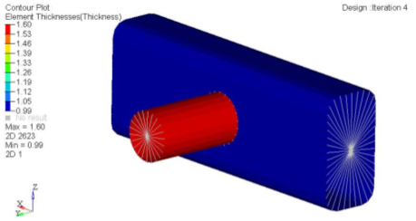
- Set the Result type to Element Thicknesses (s) and Thickness.
- Set the Averaging method to None.
- In the Results Browser, select the last load case simulation.
- In the Contour panel, click Apply.
View the Displacement Results
-
In the top, right of the application, click
 to proceed to third page.
The third page, which has results loaded from the file joint_sizeOPT_s1.h3d, is displayed. The name of the page is displayed as Subcase 1 - FORCE_X to indicate that the results correspond to subcase 1.
to proceed to third page.
The third page, which has results loaded from the file joint_sizeOPT_s1.h3d, is displayed. The name of the page is displayed as Subcase 1 - FORCE_X to indicate that the results correspond to subcase 1. - From the Animation toolbar, set the animation mode to Linear Static.
-
On the Results toolbar, click to open Contour panel.
- Set the Result type to Displacement [v] and X.
-
Click Apply.
The resulting contours represent the x component displacement field resulting from the applied loads and boundary conditions.
-
Measure the displacement at node 3143 for which you have constrained the
displacement.
-
On the Annotations toolbar, click
 to open the Measure panel.
- Click Add to add a new measure group.
- Select Nodal Contour.
- Click , then enter 3143 in the Node ID field and click OK.
The x-displacement value for 3143 (center of rigid spider, where loading is applied) displays. The x-displacement is larger than the upper bound constraint, which was defined earlier, of 0.9.Figure 3. Displacement on X-direction for the X-force loadcase at the first iteration 
-
On the Annotations toolbar, click
-
In the Results Browser, select the last iteration.
The contour now shows the x-displacement results for Subcase 1 (FORCE_X) and iteration 4, which corresponds to the end of the optimization iterations. The x-displacement is now less than 0.9.
Figure 4. Displacement on X-direction for the X-force loadcase at the last iteration 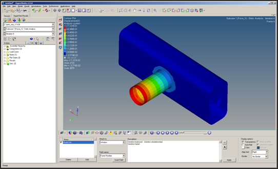
-
In the top, right of the application, click to proceed to fourth page.
The fourth page shows the results loaded from the joint_sizeOPT_s2.h3d file. The name of the page is displayed as Subcase 2 - Force_Z to indicate that the results correspond to subcase 2.
-
On the Results toolbar, click to open the Contour panel.
- Set the Result type to Displacement [v] and Z.
-
Click Apply.
The resulting contours represent the z component displacement field resulting from the applied loads and boundary conditions.
-
Measure and display the z-displacement value for node 3143.
Figure 5. 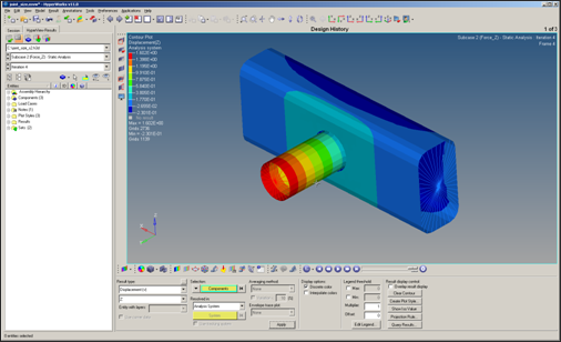
View the Gauge Thickness Results
- From the Unix or MSDOS shell, open the joint_sizeOPT.out file in a text editor.
- Review all five iterations, noting the volume, constraint information, and gauge at each iteration.
Has the volume been minimized for the given constraints?
Have the displacement constraints been met?
What are the resulting gauges for the rail and tube?