OS-T: 1500 Nonlinear Implicit Analysis of Bending of a Plate
This tutorial demonstrates nonlinear large displacement analysis in OptiStruct by simulating the bending of a plate under constant pressure.
A comparison with linear analysis results is also provided to illustrate the requirement of conducting a nonlinear large displacement analysis. This tutorial considers nonlinear geometric effects (large displacements) and elastoplastic material.
For static analysis, the energy equation reduces to F=Ku, wherein you solve for the unknown displacements (u). In Nonlinear Large Displacement analysis, the stiffness (K) may be a function of material, geometry, and boundary conditions. Therefore, an incremental-iterative approach is utilized to calculate the unknown displacements.
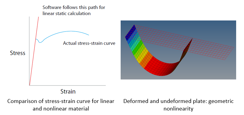
The analysis considers both geometric and material nonlinearity. The geometric nonlinearity is considered because of the large displacements observed in the geometry. Besides, the resultant stress exceeds the yield stress limit, which implies that material does not conform to a linear stress-strain behavior and plastic effects begin to be observed.
The model description is as follows:
- Units
- Length: mm
- Length
- 1000 mm
- Width
- 200 mm
- Thickness
- 4.0 mm
- Material
- Steel, elastoplastic
- Initial Density
- 7.86e-9 t/mm3
- Young's modulus (E)
- 200000 MPa
- Poisson coefficient
- 0.29
- Yield stress
- 100.0 MPa
- Tangent modulus
- 20000.0 MPa
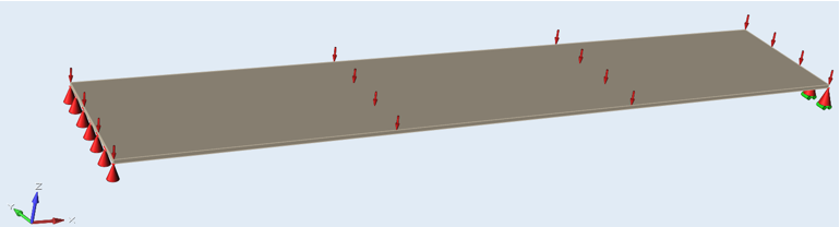
- Imposed pressure
- 0.02 MPa, applied normal to the plate
- Create plastic material and corresponding shell property
- Set up boundary conditions and imposed load
- Set up nonlinear and linear analysis
- Submit job and view results
Launch HyperMesh and Set the OptiStruct User Profile
-
Launch HyperMesh.
The User Profile dialog opens.
-
Select OptiStruct and click
OK.
This loads the user profile. It includes the appropriate template, macro menu, and import reader, paring down the functionality of HyperMesh to what is relevant for generating models for OptiStruct.
Import the Model
-
Click .
An Import tab is added to your tab menu.
- For the File type, select OptiStruct.
-
Select the Files icon
 .
A Select OptiStruct file browser opens.
.
A Select OptiStruct file browser opens. - Select the plate.fem file you saved to your working directory.
- Click Open.
- Click Import, then click Close to close the Import tab.
Set Up the Model
Update Material
- In the Model Browser, click on the material MAT1_1.
-
Input the values, as shown below. Refer to MAT1 for
more information.
Initially, the MAT1 card image represents a linear isotropic material.
-
Check the box next to MATS1 to define additional material
properties for a bilinear material elastoplastic for nonlinear analysis.
LIM1 is the material yield point, in this case, the yield stress.
H is the plasticity modulus (work hardening slope) that defines the linear relation between strain and stress in the plastic region. For a bilinear material curve, it is related to the Young’s modulus by the tangent modulus ( ). Refer to MATS1 for more information.Figure 3. Young’s and Tangent Modulus in the Stress-Strain Curve and Equation that Correlates Them 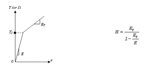
Figure 4. 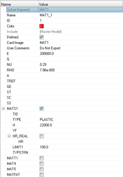
Update Property
- In the Model Browser, click on the property PSHELL_1.
-
Input the values, as shown below. Refer to PSHELL for
more information.
Figure 5. 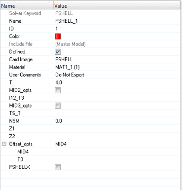
Create Boundary Conditions
- In the Model Browser, right-click and select .
- For Name, enter LC_SPC.
- Click Color and select a color from the color palette.
- For Card Image, select None.
- From the Analysis page, select constraints, toggle create.
-
Switch entity selector to nodes and select the nodes.
Figure 6. 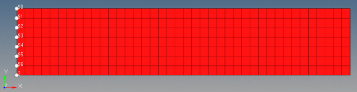
- Select the degrees of freedom dof1 and dof3. Deselect all others.
- For load types, select SPC.
- Click create to create the boundary constraints.
-
Next, select the nodesfrom opposite edge.
Figure 7. 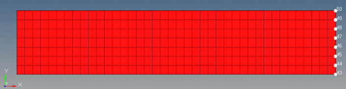
- Select the degree of freedom dof3. Deselect all others. This constrains translation movement in z direction.
- For load types, select SPC.
- Click create to create the boundary constraints.
- Click return to go back to the main menu.
Create Uniform Pressure
- In the Model Browser, right-click and select .
- For Name, enter LC_IMPLOAD.
- Click Color and select a color from the color palette.
- For Card Image, select None.
- From the Analysis page, click pressures and toggle create.
- Switch entity selector to elems and select all elements.
- Click on the toggle next to magnitute= and switch pressure defintion method to constant vector.
- For magnitude, enter -0.02.
- For load types, select PLOAD as the load type.
- Click .
Define Nonlinear Analysis Parameters
- In the Model Browser, right-click and select .
- For Name, enter LC_NLPARM.
-
For Config type, select Nonlinear Parameters.
Default type is NLPARM.
- Select DT and enter 0.0 as the value.
-
Select the CONV as UPW with an EPSUP and ESPS of
0.001, and EPSW of 1e-7, that
are the default values.
CONV flag selects the convergence criteria. In this case, UPW is a combination of displacement (U), load (P) and work (W) criteria. EPSU, EPSP and EPSW are their respective error tolerances.
-
Input the values, as shown below. Refer to NLOUT for
more information.
Figure 8. 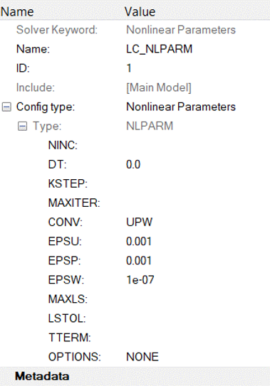
Create Output Parameters Control
- In the Model Browser, right-click and select .
- For Name, enter LC_NLOUT.
-
For Config type, select Output Parameters.
Default type will be NLOUT.
-
Check the box next to NINT and enter
10.
This parameter sets the number of intervals shown in output for intermediate results.
-
Input the values, as shown below. Refer to NLOUT for
more information.
Figure 9. 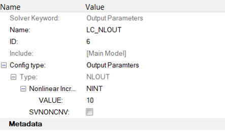
Figure 10. 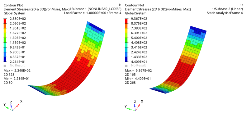
Define Output Control Parameters
- From the Analysis page, select control cards.
- Click GLOBAL_OUTPUT_REQUEST.
- For DISPLACEMENT, ELFORCE, OLOAD, STRESS, and STRAIN, set Option to Yes and click return.
- Click return twice to go to the main menu.
Activate Large Displacement Nonlinear Analysis
- From the Analysis page, select control cards.
- From control cards, select PARAM.
-
Select HASHASSM and LGDISP.
For nonlinear analysis, it is advisable to set HASHASSM card for reduction of the memory requirement and set LGDISP for activation of large displacement nonlinear static analysis.
- For HASHASSM, set Option to YES.
- For LGDISP, set to 1.
- Click return to go back to the main menu.
Create Nonlinear Static Analysis Subcase
In this step, a linear and nonlinear load case are created, both with the same boundary conditions and imposed load.
- In the Model Browser, right-click and select .
- For Name, enter nonlinear_lgdisp.
- For Analysis type, select Nonlinear static.
- For SPC, select .
-
In the Select Loadcol dialog, select
LC_SPC from the list of load collectors and click
OK.
This sets the boundary condition created above.
- For LOAD, select .
-
In the Select Loadcol dialog, select
LC_IMPLOAD from the list of load collectors and click
OK.
This sets the imposed load created above.
- For NLPARM, select .
-
In the Select Load step inputs dialog, select
LC_NLPARM from the list of load step inputs and click
OK.
This sets the analysis parameters created above.
- For NLOUT, select .
-
In the Select Load step inputs dialog, select
LC_NLOUT from the list of load step inputs and click
OK.
This sets the output control parameters created above. The nonlinear analysis has been set.
- In the Model Browser, right-click and select .
- For Name, enter linear.
- For Analysis type, select Linear Static.
- For SPC, select .
- In the Select Loadcol dialog, select LC_SPC from the list of load collectors and click OK.
- For LOAD, select .
-
In the Select Loadcol dialog, select
LC_IMPLOAD from the list of load collectors and click
OK.
The linear analysis has been set.
Submit the Job
-
From the Analysis page, click the OptiStruct
panel.
Figure 11. Accessing the OptiStruct Panel 
- Click save as.
-
In the Save As dialog, specify location to write the
OptiStruct model file and enter
plate for filename.
For OptiStruct input decks, .fem is the recommended extension.
-
Click Save.
The input file field displays the filename and location specified in the Save As dialog.
- Set the export options toggle to all.
- Set the run options toggle to analysis.
- Set the memory options toggle to memory default.
- Click OptiStruct to launch the OptiStruct job.
- plate.html
- HTML report of the analysis, providing a summary of the problem formulation and the analysis results.
- plate.out
- OptiStruct output file containing specific information on the file setup, the setup of your optimization problem, estimates for the amount of RAM and disk space required for the run, information for each of the optimization iterations, and compute time information. Review this file for warnings and errors.
- plate.h3d
- HyperView binary results file.
- plate.stat
- Summary, providing CPU information for each step during analysis process.
View the Results
- Using HyperView, open the results file (plate.out) and plot the Displacement and the von Mises stress contour at 100% load (Load Factor=1.0) for subcase 1 and subcase 2.
-
Compare the results.
Figure 13. Displacement 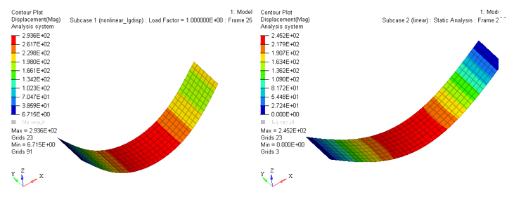
Figure 14. Stress (von Mises) 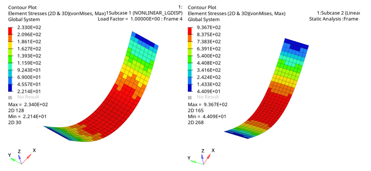
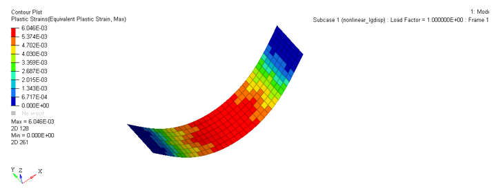
Figure 15. Plastic Strain