OS-T: 1510 Follower Loads, Nonlinear Adaptive Criteria, and Nonlinear Intermediate Results
This tutorial demonstrates how to setup Follower Loads, and the usage of Nonlinear Adaptive Criteria (NLADAPT) and how intermediate results can be requested for Nonlinear runs.
Launch HyperMesh and Set the OptiStruct User Profile
-
Launch HyperMesh.
The User Profile dialog opens.
-
Select OptiStruct and click
OK.
This loads the user profile. It includes the appropriate template, macro menu, and import reader, paring down the functionality of HyperMesh to what is relevant for generating models for OptiStruct.
Set Up the Beam Model
The beam model is a curved steel beam constructed with CHEXA elements. A Force of 100 N is applied to the top cross-section of the beam. The bottom of the beam is constrained by single point constraints (SPC).
Import the Model
-
Click .
An Import tab is added to your tab menu.
- For the File type, select OptiStruct.
-
Select the Files icon
 .
A Select OptiStruct file browser opens.
.
A Select OptiStruct file browser opens. - Select the beam_fllwer.fem file you saved to your working directory.
- Click Open.
- Click Import, then click Close to close the Import tab.
Submit the Job without Follower Loads Activation
-
From the Analysis page, enter the OptiStruct
panel.
Figure 2. Accessing the OptiStruct Panel 
-
Click save as following the input file field.
The Save As dialog opens.
-
Select the directory where you would like to write the OptiStruct model file and enter the name for the model,
beam_fllwer.fem, in the File name field.
For OptiStruct input decks, .fem is the recommended extension.
-
Click Save.
The name and location of the beam_fllwer.fem file displays in the input file field.
- Set the export options toggle to all.
- Set the run options toggle to analysis.
- Set the memory options toggle to memory default.
-
Click OptiStruct. This
launches the OptiStruct job.
If the job is successful, the new results files should be in the directory from which beam_fllwer.fem was selected. The beam_fllwer.out file is a good place to look for error messages that could help debug the input deck if any errors are present.
Set Up the Model
Activate Follower Loads
-
In the Model Browser, Cards folder, click
PARAM.
The PARAM entry is displayed in the Entity Editor.
-
Activate the Follower Loads.
- Check the box next to FLLWER.
- Set VALUE to 1.
Options 1, 2, and 3 have the same effect for concentrated loads since element face areas are not involved. Using the parameter instead of the Bulk Entry activates follower loading for all subcases in a model. If you want to only activate follower loads for specific subcases, you can use FLLWER Bulk Data and Subcase Entries.Figure 3. 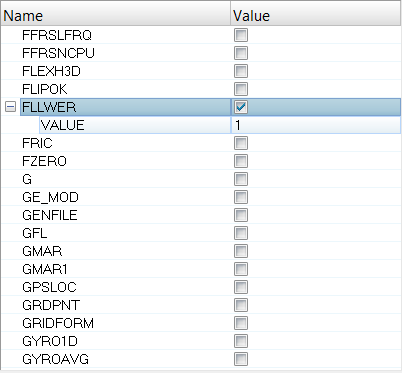
Activate Nonlinear Adaptive Criteria
-
Create a load step input.
-
Check the box next to NCUTS and enter 5
(default) in the VALUE field.
This indicates to OptiStruct that the maximum number of cutbacks allowed to reduce the time increment is 5. OptiStruct will error out if a greater number of cutbacks is required for a particular time increment for iterative convergence.
Figure 4. 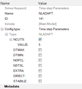
-
Check the box next to NCUTS and enter 5
(default) in the VALUE field.
-
Edit the Nonlinear Static load step.
-
Click on the field next to NLADAPT and click
LoadstepInputs.
Figure 5. 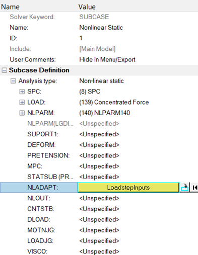
-
In the Select LoadstepInputs dialog, select
NLADAPT and click
OK.
Figure 6. 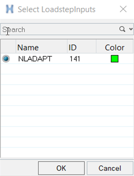
-
Click on the field next to NLADAPT and click
LoadstepInputs.
Activate Nonlinear Intermediate Results
-
Create a load step input.
-
Edit the Nonlinear Static load step.
-
Click on the field next to NLOUT, and click
LoadstepInputs.
Figure 7. 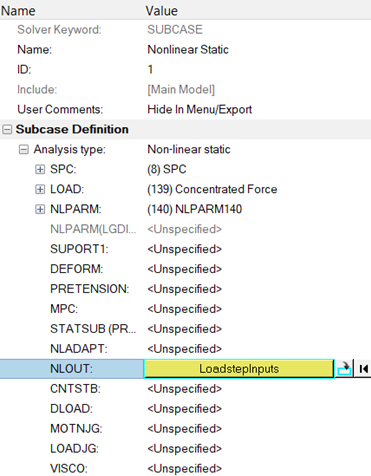
-
In the Select LoadstepInputs dialog, select
NLOUT and click
OK.
Figure 8. 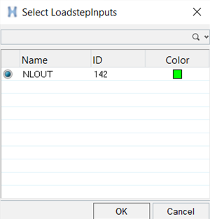
-
Click on the field next to NLOUT, and click
LoadstepInputs.
Submit the Job with Follower Loads Activation
-
From the Analysis page, enter the OptiStruct
panel.
Figure 9. Accessing the OptiStruct Panel
-
Click save as following the input file field.
The Save As dialog opens.
-
Select the directory where you would like to write the OptiStruct model file and enter the name for the model,
beam_fllwer_ON.fem, in the File name field.
For OptiStruct input decks, .fem is the recommended extension.
-
Click Save.
The name and location of the beam_fllwer_ON.fem file displays in the input file field.
- Set the export options toggle to all.
- Set the run options toggle to analysis.
- Set the memory options toggle to memory default.
-
Click OptiStruct. This
launches the OptiStruct job.
If the job is successful, the new results files should be in the directory from which beam_fllwer_ON.fem was selected. The beam_fllwer_ON.out file is a good place to look for error messages that could help debug the input deck if any errors are present.
View the Results
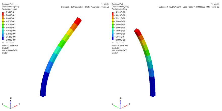
Displacements and Element Stresses are calculated by default and can be plotted using the Contour panel in HyperView.
Compare the displacement results between models without Follower Load activation.
- Launch HyperView.
-
Click
 to split the page into two windows.
-
Load the result files by clicking
 and navigating to your working directory.
- In the first window, load the beam_fllwer.h3d file.
- In the second window, load the beam_fllwer_ON.h3d file.
-
Setup contouring for each window.
-
Click the window to activate it, then click
 on the toolbar.
- Set Result type to Displacement (v).
- Click Apply.
Note: Since you have requested results for intermediate iterations via NLOUT, you will see results for all intermediate iterations. -
Click the window to activate it, then click
-
In the Results Browser, click Load
Factor and select the final increment Load Factor =
1.000000E+00.
Figure 10. 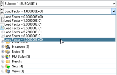
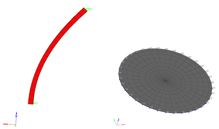
Set Up the Rubber Disk Model
The rubber disk model a rubber disk constructed with MATHE elements. A pressure load of 1 N/mm2 is applied to the rubber disk. The circumference of the disk is constrained via single point constraints (SPC).
Import the Model
-
Click .
An Import tab is added to your tab menu.
- For the File type, select OptiStruct.
-
Select the Files icon .
A Select OptiStruct file browser opens.
- Select the disk_fllwer.fem file you saved to your working directory.
- Click Open.
- Click Import, then click Close to close the Import tab.
Set Up the Model
Create Follower Load Bulk Data Entries
In the Beam model, the follower loads for concentrated forces do not depend on the area of the element face to whose grids they are applied. Therefore, the results will remain the same for any activation option chosen on either the FLLWER Bulk Data Entry or the PARAM,FLLWER entry. Additionally, since you only had one subcase, select the parameter PARAM,FLLWER to activate follower loading for this model.
- = -1, 0
- Follower force calculation is not activated.
- = 1 (default)
- Follower effect is activated. For pressure load, both element surface area and load direction are updated during the solution. For concentrated force, only the force direction is updated.
- = 2
- Follower effect is activated. For pressure load, only element surface area is updated (load direction is not updated) during the solution. For concentrated force, only the force direction is involved, which is the same as OPT = 1.
- = 3
- Follower effect is activated. For pressure load, only load direction is updated (element surface area is not updated). For concentrated force, only the force direction is updated, which is the same as OPT = 1.
-
In the Model Browser, right-click and select .
A default load collector template displays in the Entity Editor.
- For Name, enter FLLWER_1.
- Set Card Image to FLLWER.
-
Set OPT to 1.
Figure 12. 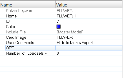
-
Create two more load collectors named FLLWER_2 and FLLWER_3.
- Set Card Image to FLLWER.
- Set OPT to 2 for FLLWER_2, and set OPT to 3 for FLLWER_3.
Reference the FLLWER Bulk Entries
The created FLLWER Bulk Data Entries should now be selected in the Subcase section.
-
Edit the fllwer_1 load step.
-
For ID, click . In the Select
Loadcol dialog, select
FLLWER_1 and click
OK.
Figure 13. 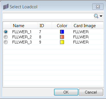
-
For ID, click . In the Select
Loadcol dialog, select
FLLWER_1 and click
OK.
-
Edit the fllwer_2 load step.
-
Edit the fllwer_3 load step.
Activate Nonlinear Intermediate Results
Parameters that allow you to activate Nonlinear Intermediate Results are available via the NLOUT Bulk Data and Subcase Entries.
The number of intervals at which intermediate results are output is controlled by the NINT parameter. The SVNONCNV parameter can be used to activate/deactivate the output of results for non-convergent solutions. This is currently turned on by default (set to YES).
-
Create a load step input.
-
Check the box next to NINT, enter 10 (Default) in the VALUE
field.
This indicates to OptiStruct that the maximum number of intervals at which intermediate results are requested is 10. If the load increment from any load "n" to load "n+1" is greater than 1/NINT (in this case, 1/10 is 0.1), then the results corresponding to load level "n+1" are saved for output; otherwise, the results are not saved.Note: This parameter has no control over the adaptive load size selection during the incremental-iterative solution process. It only specifies the number of intervals when results are saved for output during the solution process.
Figure 14. 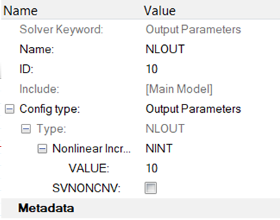
-
Check the box next to NINT, enter 10 (Default) in the VALUE
field.
-
Edit the fllwer_1 load step.
-
In the Select
LoadstepInputs dialog, select
NLOUT and click
OK.
Figure 15. 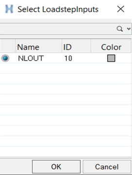
-
In the Select
LoadstepInputs dialog, select
NLOUT and click
OK.
-
Edit the fllwer_2, fllwer_3, and NO_fllwer
load steps.
Submit the Job with the Disk Model
-
From the Analysis page, enter the OptiStruct
panel.
Figure 16. Accessing the OptiStruct Panel
-
Click save as following the input file field.
The Save As dialog opens.
-
Select the directory where you would like to write the OptiStruct model file and enter the name for the model,
disk_fllwer.fem, in the File name field.
For OptiStruct input decks, .fem is the recommended extension.
-
Click Save.
The name and location of the disk_fllwer.fem file displays in the input file field.
- Set the export options toggle to all.
- Set the run options toggle to analysis.
- Set the memory options toggle to memory default.
-
Click OptiStruct. This
launches the OptiStruct job.
If the job is successful, the new results files should be in the directory from which disk_fllwer.fem was selected. The disk_fllwer_ON.out file is a good place to look for error messages that could help debug the input deck if any errors are present.
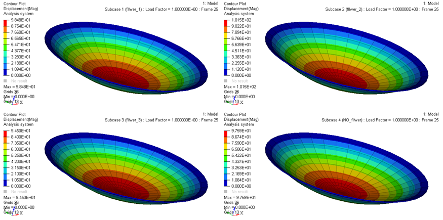
View the Results
Displacements and element stresses are calculated by default and can be plotted using the Contour panel in HyperView.
Compare the displacement results between models with and without Follower Load activation.
- Launch HyperView.
-
Click to split the page into two windows.
-
Load results from Subcase 1 to the first window.
-
Load the results file by clicking . In the panel area, load the
disk_fllwer_ON.h3d result file and click
Apply.
-
In the Results Browser, select Subcase 1
(fllwer_1) and Load Factor =
1.000000E+00.
Figure 17. 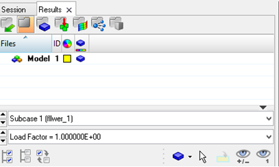
-
Load the results file by clicking
-
Load results from the remaining subcases.
- Activate the second window and load the disk_fllwer_ON.h3d result file. In the Results Browser, select Subcase 2 (fllwer_2).
- Activate the third window and load the disk_fllwer_ON.h3d result file. In the Results Browser, select Subcase 2 (fllwer_3).
- Activate the fourth window and load the disk_fllwer_ON.h3d result file. In the Results Browser, select Subcase 2 (NO_fllwer).
-
Setup contouring for each window.
-
Click the window to activate it, then click on the toolbar.
- Set Result type to Displacement (v).
- Click Apply.
Note: Since you have requested results for intermediate iterations via NLOUT, you will see results for all intermediate iterations. -
Click the window to activate it, then click