Edit Waterfall Plots
Tutorial Level: Intermediate In this tutorial, you will learn how to work with the Axes panel, query data, edit curve attributes, and use the Edit Legend dialog.
Plot attributes, such as style, color, and weight are located in the Curve Style panel. This panel also allows you to contour the surface and edit the legend, too.
Axis attributes such as labels, color, and scaling can also be modified using the Axes panel
The Values panel allows you to retrieve individual point data on any curve in the active window. When a point on a curve is selected, the point data is displayed on the panel and in a bubble in the graphics area of the screen.
Open the Session File and Create a 3D Chart Window
- From the menu bar, select .
- From the 3dplotting folder, select the file trimmer.mvw and click Open.
- Click Close on the message log that appears.
-
Create a page using the page navigation tools in the upper right corner.
Figure 4. 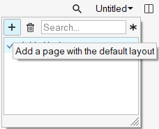
-
In the new window, click the Change Type icon (
 ) above the plot window and select 3D
Chart.
) above the plot window and select 3D
Chart.
Create a Frequency versus Time Waterfall Plot
-
From the 3D Chart ribbon, click the Waterfall tool.Figure 5. 
- Verify that Frequency and Time are the options set under Plot type:.
-
Click the curve selection button
 in the Response field for Data curves:.
- Choose the Force vs Time – Raw curve.
- Click Select.
- Verify that the curve referenced under Response is p1w2c1.
- Enter 100 for Number under Waterfall Slices.
- Check the Contour waterfall option.
-
Click Apply.
Figure 6. 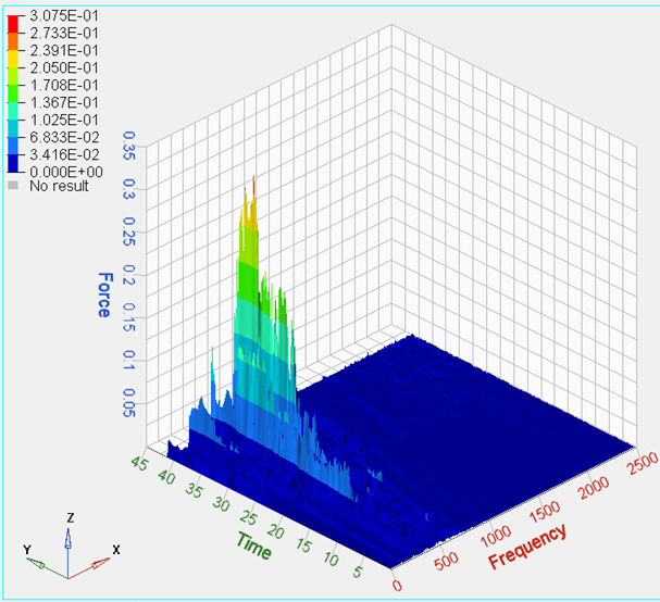
Work with the Axes Panel
-
From the 3D Chart ribbon, click the Curve Style
tool.
Figure 7. 
- Pick a color from the color palette for the X axis.
- Change the number of Tics per axis. Note what happens to the values on the X axis of the screen.
-
Click on the tabs for Y and Z
axes, respectively, and change the colors of the respective axis.
Figure 8. 
-
Click the Shading tab.
Figure 9. 
- Verify that the Grid style: is Box and change the Grid line color.
- Verify that the Axes lengths is set to Automatic.
-
Check the Lines option for Grid Style.
Figure 10. 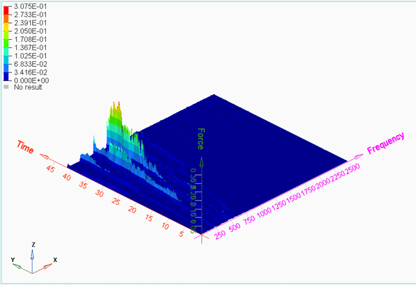
- Change the Background color by selecting a color from the palette.
- Go back to the Box option for Grid Style.
Query XYZ Values Using the Coordinate Info Panel
-
From the 3D Chart ribbon, click the Values tool.
Figure 11. 
Note: A bubble with the XYZ values is seen in the plot window. -
Click on the surface to see the XYZ values at that point.
Note: The panel area displays the XYZ values of the point chosen.
- Click Add Row to add an additional row.
-
Click on another point on the surface.
The value in the newly added row is updated to that of the new point.
-
Repeat the operation to build a table.
Figure 12. 
- Click on any one of the rows in the table and then click Remove Row.
Edit the Curve Attributes and Contour the Plot
-
From the 3D Chart ribbon, click the Curve Style
tool.
Figure 13.
- From the Curves: drop-down menu, select Waterfall.
- Verify that the Surface tab is active.
-
Change the Display mode of the surface to slices only by clicking
 from the Display mode options in the panel.
-
Change Opacity for the surface to Transparent by
clicking on
 .
.
- Change the Display mode back to waterfall as a shaded surface.
- Verify that the Contour option is active.
-
From the Expression = drop-down menu, select the X
axis.
Figure 14. 
- Repeat the previous step for the Z Axis.
Use the Edit Legend Dialog
- Click Edit legend.
-
Experiment with the following:
- Click on a number in the legend box and enter a new value.
- Press Enter.
- The edited value is displayed in bold font. The remaining values linearly interpolate.
-
Add a header and footer to the legend.
- Activate the Header check box and enter text in the text box.
-
Click the font button
 and change the font type and size.
- Click OK.
- Activate the Footer check box and enter text in the text box.
-
Click the font button and change the font type and size.
- Click OK.
- Click Apply.
-
Change the color of a legend band.
- Click on a color band.
- Select a new color.
- Click OK.
- Change another color.
-
Interpolate colors between two color bands.
- Click Interpolate.
- Click on the first changed color.
- Click on a second changed color.
- The colors between the two selected colors are interpolated.
- Click Apply.
Save Legend Settings for Future Use
Once you have completed your legend settings, you can save them for future use. Items that can be saved are listed in the Save options section.
- Activate the check boxes for the attributes you want to save.
-
Designate a file name in the Legend file field.
Files are saved in Tcl format.
- Click Save....
- Click Default to return to the default settings.
-
Click Open... to open the saved file and load the
previously determined legend settings.
The contour colors and legend are retrieved just as you saved them.