Solving a differential system of the 1st degree: Euler method

Differential systems of the 1^st degree: writing

The application of the finite element method to problems with partial derivatives of parabolic or hyperbolic type leads to solving first order differential systems of the form:

where M and N are regular matrices

Using algebraic transformations, this system can be written under the form:

(1)

Time discretization

The common principle to all numerical methods consists in the discretization of the time computation domain [t₀, t_max] into small intervals characterized by the time step Δt ≡ h.

The derivative of X(t) can be approximated by the difference between two successive in time values of X:

(2)

The tangent method

The simplest of the numerical methods, called the tangent method, consists in replacing, in the system (1), the derivative dX/dt by the precedent approximation (2).

Then, the (1) equation is written under the form:

from where the solution corresponding to the value t_i+1 = t₀ + ih of time variable is:

This method is called tangent method because it consists in determining the point (t_i+1, X_i+1) starting from the point (t_i, X_i) by using the tangent on the curve solution X(t).

Tangent method (following)

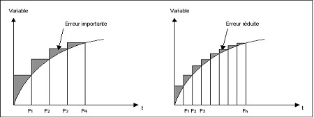
The tangent method, easy to use because of its simplicity, requires however the choice of a very small time step h in order to ensure a suitable precision of the numerical solution. The influence of the size of the time step on the precision is presented in the figure below:

Explicit / Implicit methods

Over the tangent method, more complex methods, which increase precision, are preferred. These methods allow choosing bigger time steps, the result being the decrease of the computation time.

These methods are not detailed in this document. Some data elements are proposed in the two tables below:

Method …	Description
called “of separated step” or explicit	the approximation of X at the moment t_i+1 implies only known variables at the previous moment t_i	The derivative is computed by means of the previous two steps:
called “of linked step” or implicit	the approximation of X at the moment t_i+1 implies the value of X at that moment	The derivative is computed by means of the current and the previous step:

Method …

Description

called “of separated step” or explicit

the approximation of X at the moment t_i+1 implies only known variables at the previous moment t_i

The derivative is computed by means of the previous two steps:

called “of linked step” or implicit

the approximation of X at the moment t_i+1 implies the value of X at that moment

The derivative is computed by means of the current and the previous step:

Methods…	Advantages	Disadvantages
… explicit	are easier to implement…	but often require the choice of a very small time step h because of the phenomenon of numerical instability
… implicit	are more stable and bigger time steps can be used	but require at each time step a bigger volume of computation because of the implicit term

Semi-implicit methods

In these methods, a parameter θ with its value in the range [0, 1] is introduced, and the solution corresponding to the moment t_i+1 is given by formula:

where

The values of θ which define the most used schemes are given in the following table:

Value of θ	Name of the computation scheme
1	implicit
0.878	Liniger
2/3	Galerkine
1/2	Crank-Nicholson
0	explicit

The semi-implicit methods are unconditionally stable for θ ≥ 0.5. The most used computation scheme is that known as of Crank-Nicholson that for θ = 1/2 ensures stability by giving excellent precision.

In Flux

The solved equation is a first order differential equation with respect to the time variable. This equation is integrated by an implicit method. All the quantities are computed for the final value of the time discretization interval.