Simulation Settings
The simulation can be configured by specifying the area of planning, the resolution of prediction results, prediction height and whether additional prediction planes are defined in the database.
Click to open the Edit Project Parameter dialog. The simulation settings are available on the Simulation tab.
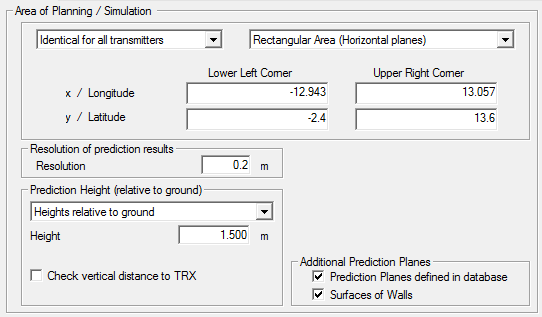
Area of Planning / Simulation
- Prediction (simulation area)
-
- Individual for each transmitter
- The simulation area can be defined as a superposition of individual prediction areas defined separately for each transmitter/cell. These individual prediction areas can be defined on the Transmitter definition tab of the corresponding transmitter.
- Identical for all transmitters
-
- Rectangular area (Horizontal planes)
- The rectangular simulation area can be specified
by defining the lower-left and upper-right corner
coordinates. Another option is to use the
 Prediction Rectangle
(Rectangle) icon on the Project
toolbar, which allows you to draw a rectangle with
the mouse.
Prediction Rectangle
(Rectangle) icon on the Project
toolbar, which allows you to draw a rectangle with
the mouse. - Multiple Points (Arbitrary Heights)
-
Specify the individual prediction / receiver , reference or user points.
- Prediction Point
- Define a point at which a prediction is to be calculated. A prediction point is indicated by a square with a red outline.
- Reference Point / Marker
- Define a point that is always visible on the
map. A reference point is indicated by a red
X
. See Balloon Markers for how to add a reference point with result value and coordinates displayed in a balloon tip. - User Point
- Define a point that represent a stationary or moving user. A user point is considered for the 5G beam switching. The name of the point can be shown/hidden, see Display Settings.
A set of prediction / receiver points can be imported from a .txt or a .csv file, and exported to a .txt file. When importing from a .csv file, a dialog will enable you to specify columns.Tip: When importing from a .csv file, you have the option to include a column with measured results. The measured results will not show up in the result tree, but a result file will be placed in the results folder. This is convenient to visualize independent results and compare them against WinProp results, for example, via menu.The prediction points can be moved by specifying a translation vector.Figure 2. The Prediction Point dialog. 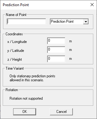
- Multiple Trajectories
-
Specify a prediction trajectory / receiver trajectory. A trajectory can be added, deleted or edited. A trajectory can be imported from a .txt or a .csv file, and exported to a .txt file. When importing from a .csv file, a dialog will enable you to specify columns. For each trajectory, specify the name, x (Longitude), y (Latitude), z (Height), Velocity, Yaw1, Pitch2 and Roll3.
Figure 3. The Trajectory dialog. 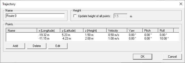
Tip: When importing from a .csv file, you have the option to include a column with measured results. The measured results will not show up in the result tree, but a result file will be placed in the results folder. This is convenient to visualize independent results and compare them against WinProp results, for example, via menu.Another option to specify a trajectory is to use the
 Prediction Trajectories
icon on the Project toolbar, which allows you to
specify the points for the trajectory using the
mouse.
Prediction Trajectories
icon on the Project toolbar, which allows you to
specify the points for the trajectory using the
mouse.
- Resolution of prediction results
- The resolution grid of the result matrix can be changed only if the database was not preprocessed in area mode. It defines the size of the result pixels used for display.
- Prediction Height
-
The height of horizontal prediction planes can be defined relative to the ground level, absolute to sea level or relative to defined floor levels.
For prediction heights relative to ground, the height of interest is location-dependent. A typical example is where a person is walking in a hilly area with a cell phone.
For prediction heights absolute to sea level, the height of interest is fixed and does not follow the terrain. A typical example is where an aircraft flies at 1500 m.
For multi-floor buildings it is possible to define multiple heights for the coverage prediction (and also network planning). In case of a high number of floors it is not required to predict the coverage of every transmitter in each floor.
For example, a transmitter in ground floor has no influence on the coverage and interference in the highest floor. To speed up the simulation in case of multi floor buildings it is now possible to define a height range (for example, 3m), so that the coverage of a transmitter is only predicted for prediction heights within the defined range (difference between z-coordinate of transmitter and prediction height are within this range).
Tip: Specify multiple prediction heights by entering space-separated values.For example:
0.5 1.5 2.5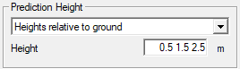
- Trajectory sampling
-
The height of a prediction trajectory can be defined relative to the ground level or absolute to sea level.
For a prediction trajectory relative to ground, the height of interest is location-dependent. A typical example is where a person is walking in a hilly area with a cell phone.
For prediction heights absolute to sea level, the height of interest is fixed and does not follow the terrain. A typical example is where an aircraft flies at 1500 m.
- Distance between evaluation points [m]
- The trajectory is sampled at the defined sampling resolution. If the distance between the defined trajectory points are larger than the specified distance between evaluation points, sampling points will be added.
- Time interval between eval. points [s]
- The trajectory is sampled at the defined time resolution.
- Add defined points and sample in between
- The defined trajectory points are used as sampling points in addition to the evaluation points.
- Additional Prediction Planes
-
ProMan also offers the possibility to do predictions on arbitrary user-defined prediction planes and on the surfaces of walls. Under Additional Prediction Planes, select the Prediction Planes defined in database check box and/or Surfaces of Walls check box.
Note: These options are only available, if the database of the current project supports this features (if this features are modeled / enabled in the database). Predictions on arbitrary predictions planes are possible using a ray-tracing model (SRT or IRT) or one of the empirical indoor wave propagation models.Figure 4. An example of predictions along building surfaces in an indoor scenario. 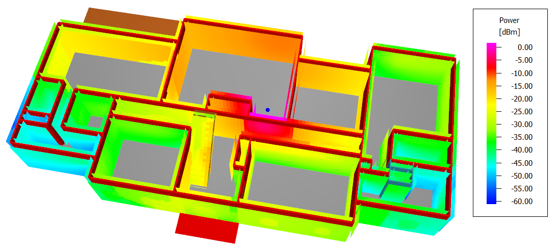
Settings related to radio network planning simulations are only available for network projects. Some of the general simulation parameters depend on the selected air interface.