Relative Heights
Calculate propagation in rural/suburban scenario with the site height set relative to ground.
Model Type
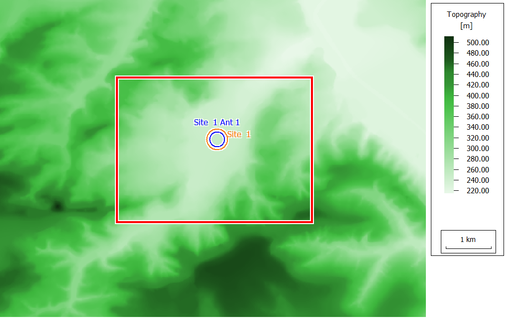
The geometry is described by topography (elevation) and is shown in Figure 1. The
Database tree enables you to view the topography (terrain
elevation at every pixel). In this example, there is no land-usage (clutter)
database. The prediction area (red rectangle) is smaller than the total available
area and as a result, reduces computation time.
Tip: Click and click the Simulation tab to set the
prediction area.
Sites and Antennas
The model contains a site with one omnidirectional antenna. The antenna is placed at
a relative height of 25 m, which is the height above ground, and operates at a
frequency of 2 GHz. The transmitter power of the antenna is 10 W.
Tip: Click and click the Sites tab to view the
antenna and site details.
Computational Method
The selected method is DPM. Contrary to
several other methods for rural propagation, DPM is a 3D deterministic method. Propagation
exponents are set to reasonable values for such a typical terrain where some of the
power is scattered by vegetation or other terrain features. Often these exponents
are fine-tuned using calibration based on a few measurements for a given
environment.
Tip: Click and click the Computation tab to set the
Path Loss Exponents.
Results
Propagation results show in every location the received power by a hypothetical
omnidirectional receiving antenna at 1.5 m above ground. The results shown below in
Figure 2 were computed
with Adaptive Resolution Management set to
Off to avoid pixels without results.
Tip: Click and click the Computation tab to set
Adaptive Resolution Management.
