Tunnel Example
Create and solve propagation inside tunnels with WinProp.
Model Overview
The model contains three subway tubes and a subway station.
TuMan
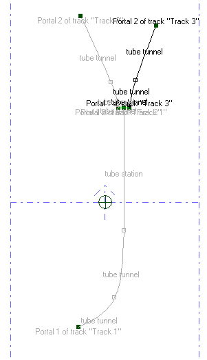
Track startpoints and endpoints are denoted portals
. A track is a tunnel which
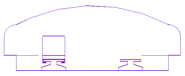
does not need to have a constant cross-section. Cross-sections are defined in
separate windows in TuMan and are assigned to segments
of the tracks. This example has two cross-sections, denoted tube tunnel
and
tube station
. The tube station is wide enough to connect to two tube
tunnels.
At the end of the TuMan session, a database is exported for use in WallMan.
WallMan
ProMan
- Sites and Antennas
-
The tunnel contains a site with two-directional radiators. The radiating antennas at a height of 5.5 m are operating on a carrier frequency of 2 GHz.Tip: Click and click the Sites tab to view the antenna settings.
- Computational Method
-
The prediction method used in this model is a 3D intelligent ray tracing model (with preprocessed data). This method requires a preprocessed geometry database. Result resolution and prediction height were defined during preprocessing.Tip: Click and click the Computation tab to view the method.
- Results
-
Propagation results show at every location the power received from each individual transmitter antenna. Figure 4 shows the results for Site 1 Antenna 1 at a height of 4 m (a predefined height).
Figure 4. Power received by a hypothetical isotropic antenna when antenna 1 is transmitting. 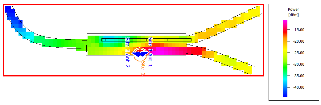
Propagation results were calculated for field strength, path loss, delay spread, and angular spreads.