Tutorial Level: Beginner Run a baseline static analysis, then review and animate the results.
In this lesson you will learn how to:
Open a model and display the Model Browser
Run a baseline static analysis
View results for the factor of safety
View results for displacement
View results for von Mises stress
View results for tension and compression
Play an animation
Overview
In this tutorial, you will run a baseline static analysis of a part in a steady state
and review the results.
In mechanics, when the loading on a system is balanced, we achieve equilibrium, or a
steady state. Analysis performed at this state is also called static analysis. When
solving a static analysis, the solvers will solve the equation Kx = f where:
K: is the global stiffness matrix
x: is the displacement vector response to be determined
f: is the external forces vector applied to the structure
The following tutorial demonstrates how to run a baseline analysis in order to better
understand what a static analysis is.
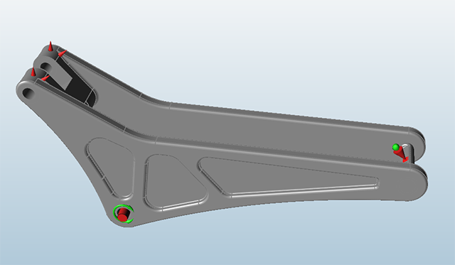
Open the Baseline Analysis Model
Before you begin, copy the file(s) used
in this tutorial to your working directory.
Double-click the Baseline Analysis.stmod file to load it
in the modeling window.
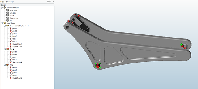
If not already visible, press F2 to open the Model Browser.
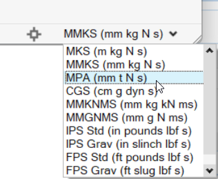
Make sure the display units in the Unit System Selector are set to
MPA (mm t N s).
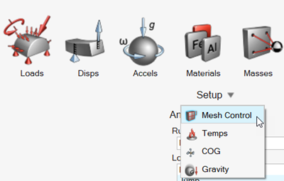
Run a Baseline Static Analysis
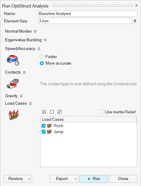
On the Structure ribbon, click the Run Analysis button in the Analyze tool
group to open the Run Analysis window.
Run the analysis using the following settings:
Select OptiStruct as the solver.
Change the Element Size to 3.0
mm.
Set Speed to More
Accurate.
Click Load Cases and verify that both the
Jump and the Rock load
cases are selected.
Click Run to perform the analysis.
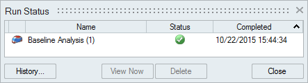
When the run is complete, select it in the Run Status window and click
View Now to see the results.
Tip: You can also
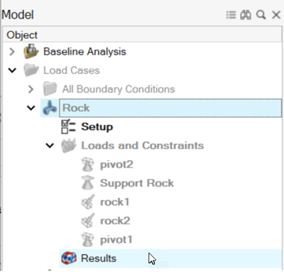
double-click the Results icon in the Model Browser to
view results for a load case.
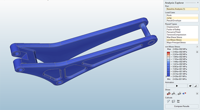
The results are displayed in the Analysis Explorer.
View the Factor of Safety Results
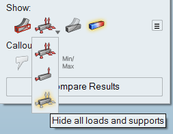
In the Analysis Explorer, click Show Selected Load Case and select Hide all Loads and
Supports.
In the Analysis Explorer under Load Case, select
Jump.
In the Analysis Explorer under Result Types, select
Factor of Safety. The Factor of Safety result type
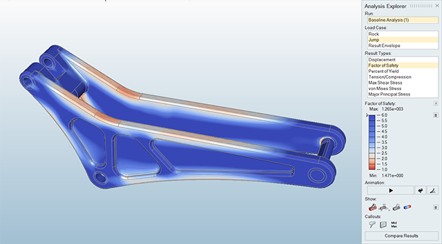
for the Rock load case is shown in the modeling window.
By default, areas that are approaching a minimum safety factor of 1.0 are
shown in red to indicate where the part is most likely to fail. The areas shown
in pink indicate where the model is under stress.
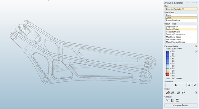
In the Analysis Explorer under Factor of Safety, click
and drag the slider on the legend until just before the contours
disappear.
This masks all areas on the model with a factor of safety higher than the
selected value on the slider.
The factor of safety is around 1.7. Since this is greater than 1.0, the model
is not predicted to fail for this load case.
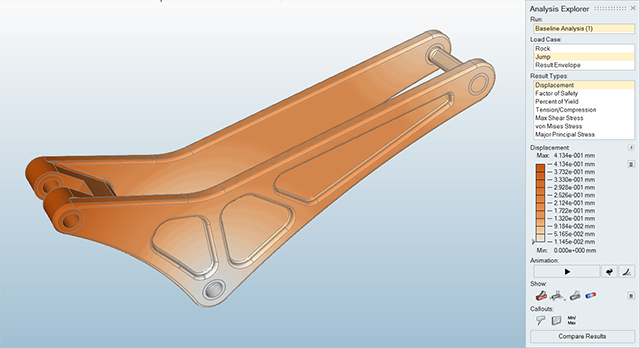
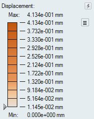
View the Displacements Results
In the Analysis Explorer under Result Types, select
Displacement.
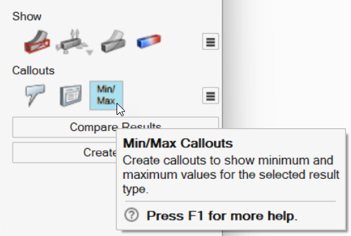
Turn on the Min/Max callout and note that the maximum
displacement for the model is approximately .396 mm as shown in the
legend.
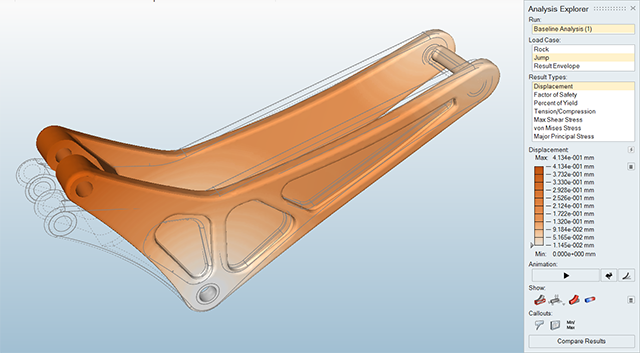
Click Show/Hide Deformed State to show the deformed state of the model. Click
again to hide it.
Click the button on the animation toolbar to visualize the
displacement. Click the button to pause
the animation.
Optional: Click the icon to change the
animation settings.
Tip:Inspire automatically scales the displacement
animation to make it easier to see. Deselect the Auto
checkbox and enter a Scale By value to change the
scale of the animation.
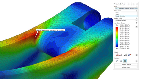
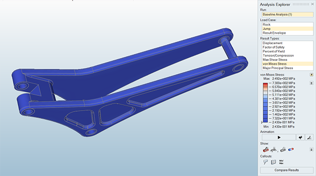
View the von Mises Stress Results
With the Jump load case still selected, select
von Mises Stress under Result
Types.
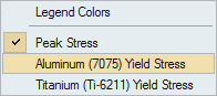
By default, the peak stress for the load case is shown. Click next to the legend in the Analysis Explorer and
select Aluminum (7075) Yield Stress.
The majority of the rocker arm is blue, but the pin is red. However, the pin is
made of titanium, not aluminum.
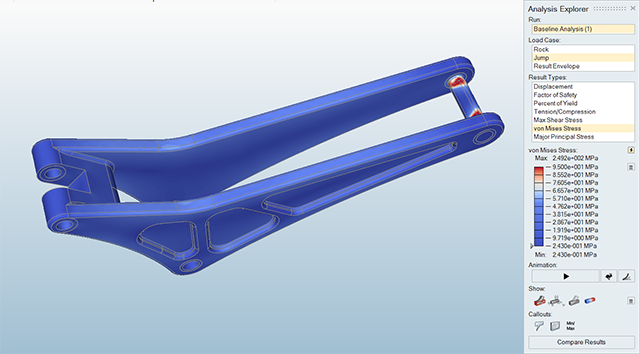
Click next to the legend in the Analysis Explorer and
select Titanium (Ti -6211 Yield Stress).
Now the pin is blue as well. It's looking good!
Tip: If you want
to change the legend colors used for this or any other result type, click
Legend Options next to the legend and select
Rainbow Legend colors. Alternatively, you can use Preferences > Inspire > Run Options > Analysis Legend Colors to change the default legend colors for each result
type.
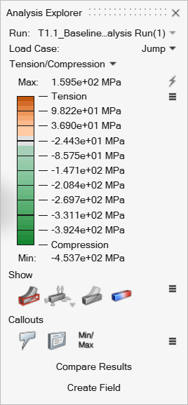
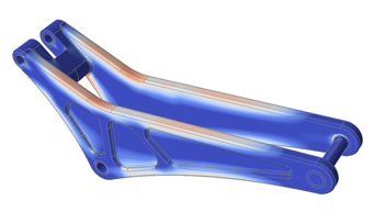
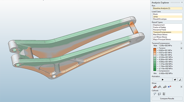
View the Tension and Compression Results
Select Tension/Compression under Result
Types.
Areas on the model shown in orange are subject to tension, and areas
shown in green are subject to compression.
Click Show/hide initial shape to show and hide the initial shape as a
reference.
Click Show/hide contours to show and hide the
contours. Use Show/Hide Options to turn off
Blended contours and Interpolate during
animation.
Optional: If you want to change the maximum value in the legend, double-click the label
for the maximum value and type a new value. Analysis results are updated after
you press Enter.
Optional: If you want to change the legend colors used for this or any other result type,
click Legend Options next to the legend and select Rainbow
Legend colors. Alternatively, you can use Preferences > Inspire > Run Options > Analysis Legend Colors to change the default legend colors for each result type.
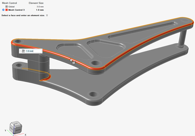
Select the highlighted surfaces and define the mesh size on these surfaces as
1.0 mm. This will seed the underlying solid mesh with
a smaller element size than the global value of 3.0 mm.
Note: Hold down Ctrl to select
multiple faces.
On the Structure ribbon, click the Run Analysis button in the Analyze tool
group to open the Run Analysis window.
Rerun the analysis using the following settings:
Change the Element Size to 3.0
mm.
Select OptiStruct as the solver.
Set Speed to More
Accurate.
Click Load Cases and verify that both the
Jump and the Rock load
cases are selected.
Click Run to perform the analysis.
When the run is complete, select it in the Run Status window and click
View Now to see the results.
Tip: You can also
double-click the Results icon in the Model Browser to
view results for a load case.
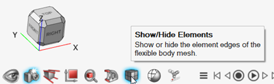
Select Show/Hide Elements in the View Controls to show
the mesh.
Note the mesh refinement on the selected fillets and the smoother transition
of stress results.

 button in the Analyze tool
group to open the Run Analysis window.
button in the Analyze tool
group to open the Run Analysis window.

 The results are displayed in the Analysis Explorer.
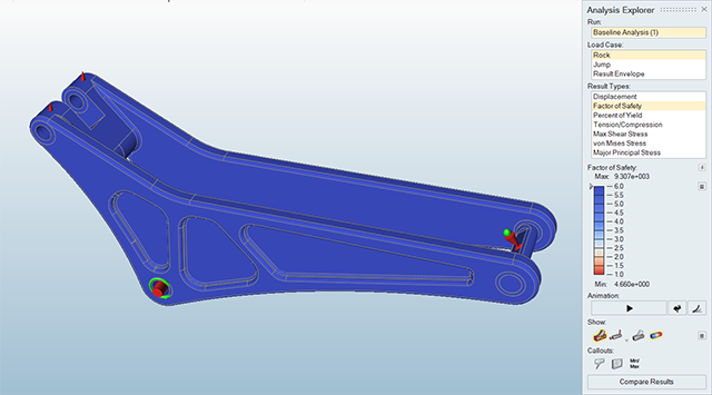
 and select Hide all Loads and
Supports
and select Hide all Loads and
Supports
 .
.
 to show the deformed state of the model. Click
again to hide it.
to show the deformed state of the model. Click
again to hide it.
 button on the animation toolbar to visualize the
displacement. Click the
button on the animation toolbar to visualize the
displacement. Click the  button to pause
the animation.
button to pause
the animation.
 icon to change the
animation settings.
icon to change the
animation settings.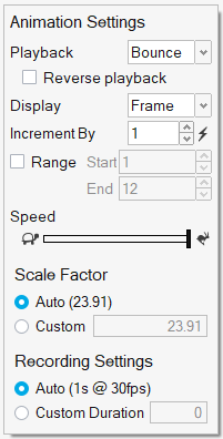
 next to the legend in the Analysis Explorer and
select Aluminum (7075) Yield Stress.
next to the legend in the Analysis Explorer and
select Aluminum (7075) Yield Stress.
 to show and hide the initial shape as a
reference.
to show and hide the initial shape as a
reference.
 to show and hide the
contours. Use Show/Hide Options
to show and hide the
contours. Use Show/Hide Options