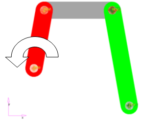
The mass of the system is to be minimized by controlling 12 shape design variables
while the stress should be less than an allowable value. Left link is a driving link
whose angular velocity is 50 rad/sec. Units (kg, N, cm, s).Figure 1. 4 Bar Linkage
The optimization problem for this tutorial is stated as:
Objective
Minimize mass.
Constraints
Upper bound on stress.
Design Variables
Shape design variables of the three flexible bodies.
Launch HyperMesh and Set the OptiStruct User Profile
Launch HyperMesh.
The User Profile dialog opens.
Select OptiStruct and click
OK.
This loads the user profile. It includes the appropriate template, macro
menu, and import reader, paring down the functionality of HyperMesh to what is relevant for generating models for
OptiStruct.
Open the Model
Click File > Open > Model.
Select the 4bar_design.hm file you saved to
your working directory.
Click Open.
The 4bar_design.hm database is loaded
into the current HyperMesh session, replacing any
existing data.
Set Up the Model
Define a Driving Motion
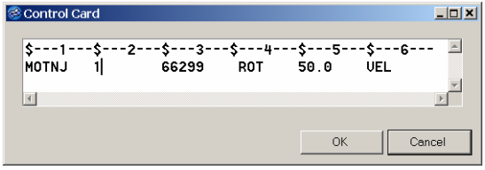
In this tutorial, the driving motion at a joint, MOTNJ is defined.
However, MOTNJ is not currently supported by HyperMesh, so the card needs to be entered manually.
From the Analysis page, click the control cards
panel.
In the Card Image dialog, click
BULK_UNSUPPORTED_CARDS.
In the Control Card dialog, enter the following and click
OK.
Figure 2. Constant velocity (50 Rad/s) applied to the joint 66299
Click return.
Update Boundary Conditions and MOTION
In the Model Browser, Load Steps folder, click
SUBCASE1.
The Entity Editor opens and displays the load
steps card details.
Set the Analysis type to Multibody dynamics.
For MBSIM, select MBSIM1.
Select SUBCASE_UNSUPPORTED.
Click
and enter MOTION = 1.
Submit the Job
From the Analysis page, click the OptiStruct
panel.
Figure 3. Accessing the OptiStruct Panel
Click save as.
In the Save As dialog, specify location to write the
OptiStruct model file and enter
4bar_design_analysis for filename.
For OptiStruct input decks,
.fem is the recommended extension.
Click Save.
The input file field displays the filename and location specified in the
Save As dialog.
Set the export options toggle to all.
Set the run options toggle to analysis.
Set the memory options toggle to memory default.
Click OptiStruct to launch
the OptiStruct job.
If the job is successful, new results files
should be in the directory where the 4bar_design_analysis.fem was written. The 4bar_design_analysis.out file is a good place to look for error messages that could help
debug the input deck if any errors are present.
View the Results
From the OptiStruct panel, click HyperView.
HyperView is launched and the results are
loaded. A message window appears to inform of the successful model and result
files loading into HyperView.
On the Results toolbar, click to open the
Contour panel.
Set the Result type to Element Stresses (2D & 3D)
(t).
Click Apply.
Click the Legend tab.
Click Edit Legend.
Set the Type to Dynamic scale.
Other properties can be changed here to created the desired legend.
On the Page Controls toolbar, set the page layout to , which create two vertical windows.
Click the second window to make it active.
From the client selector, select (HyperGraph 2D).
Click the first window to make it active.
On the Annotations toolbar, click to open the Measure panel.
In the Measure Groups list, select Dynamic MinMax
Result.
From the list below Resolved in , click Max.
Click Create Curve.
Set Place curve on: to Existing Plot.
A list of plot windows on this report are exposed.
Select Live link.
Click window 2 to make it active.
Click Apply.
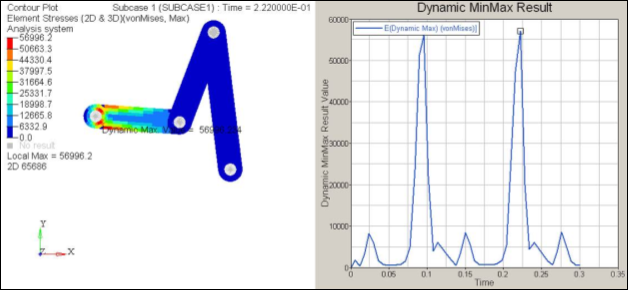
The Maximum von Mises stress (t) is plotted.Figure 4. MBD Stress results (Max = 56996 N/cm2)
Save the file as a template to be applied on the optimization results.
From the menu bar, click File > Save As > Session.
In the Save Session As dialog, save the file as
Stress_report.tpl.
In the top, right of the application, click / to
return to Page 1 and the HyperMesh client.
Set Up the Optimization
Create Boundary Conditions for Structural Analysis
Structural analysis and optimization of the flexible bodies of this model are performed
in ESL optimization. Thus, the boundary condition for the flexible bodies needs to be
defined.
Create the load collector, BCforOpt.
In the Model Browser, right-click and select Create > Load Collector from the context menu.
A default load collector displays in the Entity Editor.
For Name, enter BCforOpt.
Click Color and
select a color from the color palette.
Set Card Image to None.
Enable coincident picking.
From the menu bar, click Preferences > Graphics.
Select coincident picking.
Click return.
Create constrains.
From the analysis page, click the constraints
panel.
Select all dofs (1 through 6).
All of the dofs (1 through 6) should be fixed to remove the 6 rigid
body motion of each flexible body. Make sure that dof1 through dof6 are
all checked in the constraints panel.
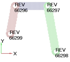
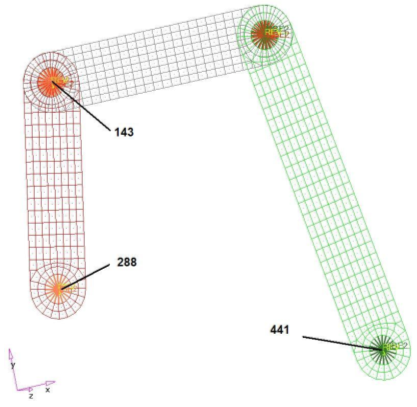
Click the center of the lower spider of the component Left. You should
see two node numbers at one location; choose node
288.
Click the center of the left spider of the component Middle and choose
node 143.
Click the center of the lower spider of the component Right and choose
node 441.
Set load type to SPC.
Click create.
Figure 5. Nodes to be constrained to arrest rigid body motions
Update Boundary Condition and MOTION in the Predefined MBD Subcase
In the Model Browser, Load Steps folder, select
SUBCASE1.
The Entity Editor opens and displays the load
steps card details.
Set the Analysis type to Multi-body dynamics.
For MBSIM, select MBSIM1.
For SPC, select BCforOpt.
Define Shape Design Variables
The shape perturbation vectors already have been created in this database. For more details
about creating shape perturbation vectors, refer to other tutorials related to HyperMorph. In this step, you will define shape design variables
with the predefined shape perturbation vectors.
From the Analysis page, click the optimization
panel.
Click the shape panel.
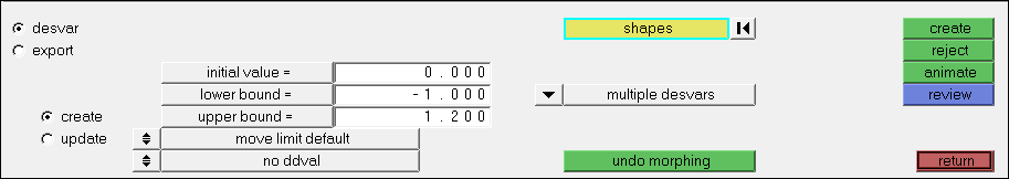
Select the desvar subpanel.
Switch from single desvar to multiple desvars.
Using the shapes selector, select all shapes.
In the lower bound= field, enter -1.0.
In the upper bound= field, enter 1.2.
Figure 6.
Click create.
Click return to go to the optimization panel.
12 shape design variables are created.
Create Optimization Responses
From the Analysis page, click optimization.
Click Responses.
Create the mass response, which is defined for the total volume of the
model.
In the responses= field, enter mass.
Below response type, select mass.
Set regional selection to total and
no regionid.
Click create.
Create a static stress response.
In the response= field, enter Stress.
Set the response type to static stress.
Using the props selector, select Middle, Left, Right.
Set the response selector to von mises.
Under von mises, select both surfaces.
Click create.
Click return to go back to the Optimization panel.
Define the Objective Function
Click the objective panel.
Verify that min is selected.
Click response and select Mass.
Click create.
Click return twice to exit the Optimization panel.
Create Design Constraints
Click the dconstraints panel.
In the constraint= field, enter Constr.
Click response = and select Stress.
Check the box next to upper bound, then enter
30000.
Using the loadsteps selector, select SUBCASE1.
Click create.
Click return to go back to the Optimization panel.
A constraint is defined on the response Stress. The constraint will
force the maximum stress on SUBCASE1 to be less than 30000.0 N/cm2.
Run the Optimization
From the Analysis page, click OptiStruct.
Click save as.
In the Save As dialog, specify location to write the
OptiStruct model file and enter
4bar_design_opt for filename.
For OptiStruct input decks,
.fem is the recommended extension.
Click Save.
The input file field displays the filename and location specified in the
Save As dialog.
Set the export options toggle to all.
Set the run options toggle to optimization.
Set the memory options toggle to memory default.
Click OptiStruct to run the optimization.
The following message appears in the window at the completion of the
job:
OPTIMIZATION HAS CONVERGED.
FEASIBLE DESIGN (ALL CONSTRAINTS SATISFIED).
OptiStruct also reports error messages if any exist. The
file 4bar_design_opt.out can be opened in a
text editor to find details regarding any errors. This file is written to the
same directory as the .fem file.
Click Close.
View the Results
View Stress Results
From the OptiStruct panel, click HyperView.
HyperView is launched and the results are
loaded. A message window appears to inform of the successful model and result
files loading into HyperView.
Open the report template, Stress_report.tpl.
From the menu bar, click File > Open > Report Template.
In the Open Report File dialog, open the
Stress_report.tpl file.
For GRAPHIC_FILE_1 and RESULT_FILE_1, select 4bar_design_opt_mbd_0#.h3d from where the optimization
was run (the highest # should be the final iteration).
A message appears explaining that the Element Stresses (2D & 3D)
results do not exist - this is because the stress results on MBD simulations are
just named Stress.
Close the Message Log window.
Click on window 1 to make it current.
On the Results toolbar, click to open the
Contour panel.
Set the Result type: to Stress (t).
Click the traffic light icon to start the
animation.
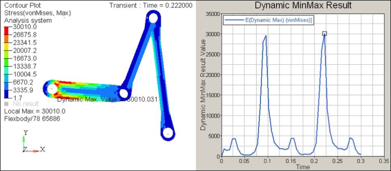
Figure 7. von Mises stress contour (Max < 30000 N/cm2)
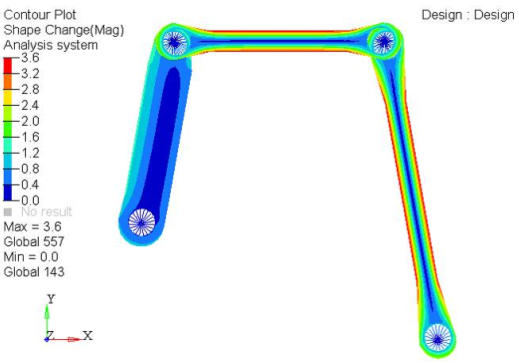
Contour the Shape Change
On the Page Controls toolbar, click to add a new page to the session.
On the Standard toolbar, click and open the last iteration
(highest) number result file of 4bar_design_opt_des_0#.h3d from where the optimization was run.
Click Apply.
On the Results toolbar, click to open the
Contour panel.
Set the Result type: to Shape Change (v).
Click Apply.
Figure 8. Shape changing contour
Open the file 4bar_design_opt.dsvar to see how
OptiStruct changed the DVs during the optimization
process.
This will show that all DVs for the right and mid arms went to the limit of 1.2,
showing that minimizing the mass of these two arms are key to reducing the
Stress.

 and enter MOTION = 1.

 to open the
Contour panel.
to open the
Contour panel.
 , which create two vertical windows.
 (HyperGraph 2D).
 to open the Measure panel.
 /
/ to
return to Page 1 and the HyperMesh client.
to
return to Page 1 and the HyperMesh client.
 to add a new page to the session.
 and open the last iteration
(highest) number result file of 4bar_design_opt_des_0#.h3d from where the optimization was run.
and open the last iteration
(highest) number result file of 4bar_design_opt_des_0#.h3d from where the optimization was run.