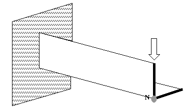
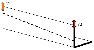
In the schematic, the vertical deflection at point N should be limited to 2.0mm while
minimizing the amount of material required.Figure 1. Cantilever L-Beam Schematic
The optimization problem for this tutorial is stated as:
Objective
Minimize mass.
Constraints
A given maximum nodal displacement < 2 mm.
Design Variables
Shape of each of the beam flanges.
Launch HyperMesh and Set the OptiStruct User Profile
Launch HyperMesh.
The User Profile dialog opens.
Select OptiStruct and click
OK.
This loads the user profile. It includes the appropriate template, macro
menu, and import reader, paring down the functionality of HyperMesh to what is relevant for generating models for
OptiStruct.
Open the Model
Click File > Open > Model.
Select the Lbeamshape.hm file you saved to
your working directory.
Click Open.
The Lbeamshape.hm database is loaded
into the current HyperMesh session, replacing any
existing data.
Set Up the Optimization
Create Shapes with HyperMorph
From the Analysis page, click the optimization
panel.
Click the HyperMorph panel.
Create domains and handles.
Click the domains panel.
Select the create subpanel.
Set the switch to auto functions.
Click generate.
Click return to return to the HyperMorph panel.
A number of domains and handles are created which will enable us to morph the
shape of the beam.
There are two types of handles; global handles, which are represented by
larger red balls and local handles, which are represented by smaller yellow
balls. Only local handles are available in this tutorial.
Move handles.
Click the morph panel.
Select the move handles subpanel.
Switch from interactive to translate.
Using the handles subpanel, select the local handle that is located at
the node where the load is applied.
Note: Local handles are indicated by a yellow ball.
In the y val= field, enter -10.0.
Click morph.
The beam changes shape so that the handle you selected moved -10.0 in
the y-direction. Note how the mesh adjusted to this change in
shape.
Save the shape.
Select the save shape subpanel.
In the name= field, enter shape1.
Click color and select a color for the shape.
Under shape=, select as node
perturbations.
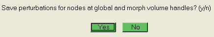
Click save.
Click Yes to the message regarding the
perturbations.
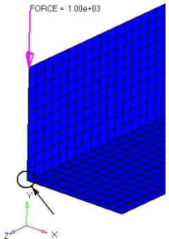
Figure 2.
This shape is saved as shape1. Later, you can associate it to a design
variable.
Click undo all.
The model returns to its original shape.
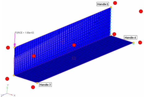
Repeat steps 4 and 5 for the local handles 3, 4 and 5.
Translate handles 3 and 4 by x=-10 and handle 5 by y=-10.
Save the shapes after morphing each handle as shape2, shape3 and
shape4, respectively.
Figure 3. Handles to be Morphed
Click return twice to go to the Optimization panel.
Create Shape Optimization Design Variables
Click the shape panel.
Select the desvar subpanel.
Toggle the switch from single desvar to multiple
desvars.
Using the shapes selector, select shape1,
shape2, shape3, and
shape4.
Click create.
Click return to go to the optimization panel.
Four shape design variables are created using the shapes that were saved earlier.
A potential variation in shape of the vertical flange of the L-beam that could be
achieved using the set up described.Figure 4.
Create Optimization Responses
From the Analysis page, click optimization.
Click Responses.
Create the mass response, which is defined for the total volume of the
model.
In the responses= field, enter Mass.
Below response type, select mass.
Set regional selection to total and
no regionid.
Click create.
Create the displacement response.
In the response= field, enter Disp.
Below response type, select static
displacement.
Using the nodes selector, select the response node.
Set the displacement type to dof2.
dof1, dof2, dof3
Translation in the X, Y, and Z directions.
dof4, dof5, dof6
Rotation about the X, Y, and Z axes.
total disp
Resultant of the translational displacements in x, y, and z
directions.
total rotation
Resultant of the rotational displacements in x, y, and z
directions.
Click create.
Figure 5.
Click return to go back to the Optimization panel.
Define the Objective Function
Click the objective panel.
Verify that min is selected.
Click response and select mass.
Click create.
Click return twice to exit the Optimization panel.
Create Design Constraints
Click the dconstraints panel.
In the constraint= field, enter constr.
Click response = and select Disp.
Check the box next to lower bound, then enter
-2.0.
Using the loadsteps selector, select load.
Click create.
Click return to go back to the Optimization panel.
Save the Database
From the menu bar, click File > Save As > Model.
In the Save As dialog, enter lbeamshape_opt.hm for the file name and save it to your
working directory.
Run the Optimization
From the Analysis page, click OptiStruct.
Click save as.
In the Save As dialog, specify location to write the
OptiStruct model file and enter
lbeamshape_opt for filename.
For OptiStruct input decks,
.fem is the recommended extension.
Click Save.
The input file field displays the filename and location specified in the
Save As dialog.
Set the export options toggle to all.
Set the run options toggle to optimization.
Set the memory options toggle to memory default.
Click OptiStruct to run the optimization.
The following message appears in the window at the completion of the
job:
OPTIMIZATION HAS CONVERGED.
FEASIBLE DESIGN (ALL CONSTRAINTS SATISFIED).
OptiStruct also reports error messages if any exist. The
file lbeamshape_opt.out can be opened in a
text editor to find details regarding any errors. This file is written to the
same directory as the .fem file.
Click Close.
View the Results
View the Deformed Structure
It is helpful to view the deformed shape of a model to determine if the boundary conditions
have been defined correctly and also to check if the model is deforming as
expected. In this section, use the Deformed panel to review the deformed
shape for the last design iteration and a scale factor, and overlay the
undeformed shape.
From the OptiStruct panel, click
HyperView.
HyperView launches within
the HyperMesh Desktop and loads
.h3d files that contain
optimization results on page 2 and analysis results on page
3.
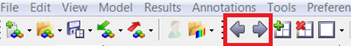
In the top, right of the application, use the navigations
buttons to navigate to the Design History (page 2).
Figure 6.
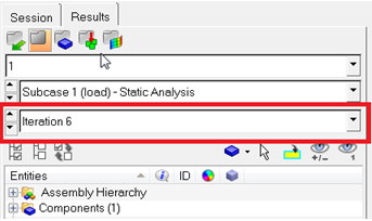
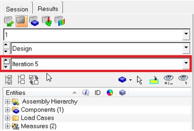
In the Results Browser, select the last
iteration (iteration 6).
Figure 7.
On the Results toolbar, click to open the Contour panel.
Set the Result type: to Shape change
(v).
Click Apply.
The final shape for the Iteration # can now be seen.
View a Transient Animation of the Shape Contour Changes
On the Animation toolbar, click to start the animation.
The seek slider and playback speed slider (top and bottom
respectively) are located next to the playback controls.Figure 8.
Move the speed slider to adjust the animation speed.
After reviewing the animation, click to stop the animation.
Move the Current time: back to 0.
Plot a Displacements Contour
In the top, right of the application, click to go to page 3, which contains the analysis
results.
On the Results toolbar, click to open the Contour panel.
Set the Result type: to Displacement (v)
and Y (Y component of the
Displacement, which is what was constrained).
In the Results Browser, select the last
iteration (iteration 6).
Figure 9.
Click Apply.
A plot of the displacements on your final shape displays. The maximum
displacements for the last Iteration #, is still below 2.0.

 to open the Contour panel.
 to start the animation.
The seek slider and playback speed slider (top and bottom respectively) are located next to the playback controls.
to start the animation.
The seek slider and playback speed slider (top and bottom respectively) are located next to the playback controls.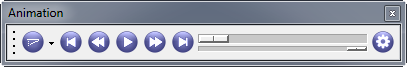
 to stop the animation.
 to go to page 3, which contains the analysis
results.
to go to page 3, which contains the analysis
results.