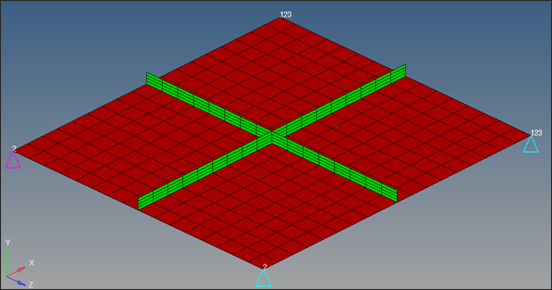
A global search approach will be used to generate the multiple starting points. The
structure, consisting of one base panel and the cross shaped ribs, is subjected to a
frequency-varying unit load excitation using the modal method. The goal is to
achieve the best stiffened structure by changing the shapes of the ribs.Figure 1. Model Review
A regular shape optimization has been defined in the model. The formulation of this
optimization is stated as:
Objective
Minimize the maximum (minmax) displacement at the node where the
excitation load was applied.
Constraints
Mass < 2.0e-3.
Design Variables
Shape design variables.
Launch HyperMesh and Set the OptiStruct User Profile
Launch HyperMesh.
The User Profile dialog opens.
Select OptiStruct and click
OK.
This loads the user profile. It includes the appropriate template, macro
menu, and import reader, paring down the functionality of HyperMesh to what is relevant for generating models for
OptiStruct.
Import the Model
Click File > Import > Solver Deck.
An Import tab is added to your tab menu.
For the File type, select OptiStruct.
Select the Files icon .
A Select OptiStruct file browser
opens.
Select the rib_opt.fem file you saved
to your working directory.
Click Open.
Click Import, then click Close to
close the Import tab.
Review the Model and Optimization Setup
The shape optimization of the frequency response model has been defined in the model.
In the Model Browser, review the model, loadstep, and
optimization setup.
Figure 2.
From the Analysis page, click the optimization
panel.
Click the shape panel to review the shape design
variables.
Click animate.
One of the shapes should be displayed in the simulation=
field.
Click linear.
The animation of that shape displays.
Review the other shapes by clicking next or
prev.
Click return to go back to the Optimization panel.
Initiate the Run
From the Analysis page, click the OptiStruct
panel.
The name and location of the rib_opt.fem file displays in the input file: field. The location where
the model and result files will be written can be modified.
Click OptiStruct.
After the running process completes, go to the working directory and open the
rib_opt.out file. Check the
optimization history and the final optimal design.
Go back to the Analysis page.
Define the DGLOBAL Cards
From the Analysis page, click the control cards
panel.
In the Card Image dialog, click
CASE_UNSUPPORTED_CARDS.
In the Control Card dialog, enter
DGLOBAL=1 and click OK.
Click BULK_UNSUPPORTED_CARDS.
In the Control Card dialog, enter
DGLOBAL,1 and click OK.
Click return.
Both Subcase and Bulk Data Entries for global search are created with default
parameters.
Initiate the Run
From the Analysis page, click the OptiStruct
panel.
The name and location of the rib_opt_global.fem file displays in the input file: field. The location where
the model and result files will be written can be modified.
Click OptiStruct.
After the running process completes, go to the working directory and open the
rib_opt_global.out file. Check the
optimization history and the final optimal design.
Go back to the Analysis page.
View the Results
Post-process the GSO Results
Since the default parameters are used for GSO, OptiStruct
determines the number of starting points and number of groups of design variables
automatically.
Open the rib_opt_global.out file.
A general summary of the GSO run is output at the end of the out file.
This GSO run completed with 20 starting points. Seventeen (17) unique designs
were found, which means three designs were repeated. The best design was found
at starting point 3. The table of unique designs and table of designs were also
printed with the information of starting point, objective function, constraint
violation, times found, and directory suffix.
Compare the best design with the results from the regular optimization
approach.
In the working directory, 17 directories with suffix
'_GSO_V1_V2' were created for the unique designs. V1 is
the number of the starting point, and V2 is the rank of this design among all
unique designs. The optimization results of each starting point can be found in
the directory, respectively.
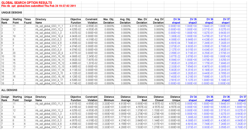
Open the Excel file, rib_opt_global_GSO.slk.
The tables for unique designs and all designs are printed in the Excel
file. The best design among the GSO runs was achieved with the 3rd starting
point, and the results of this design were saved in the directory,
rib_opt_global_GSO_3_1, and this design was found three
times during the global search. In GSO search, if the difference between two
designs is under the unique design tolerance, they are considered identical; for
example, the designs with starting points 11 and 3. This information can be
found in the table of all designs. The statistical information and the optimal
design variables for each run are also available.Figure 3.
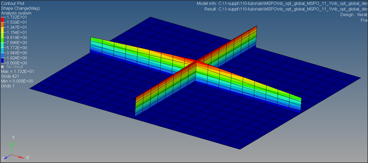
Post-process the Best Design
The following steps demonstrate how to review the best design of GSO in
HyperView.
In the OptiStruct panel, click HyperView.
In the Load Results panel, load the rib_opt_global_des.h3d
file located in the /rib_opt_global_GSO_3_1
directory.
Click Apply.
The h3d file containing optimization results is loaded.
In the Results Browser, select Iteration
10.
On the Results toolbar, click to open the
Contour panel.
Set the Result type to Shape Change (v).
Click Apply.
The optimized shape at the final iteration displays.Figure 4. Best Optimized Shape Design from GSO

 .
A Select OptiStruct file browser opens.
.
A Select OptiStruct file browser opens.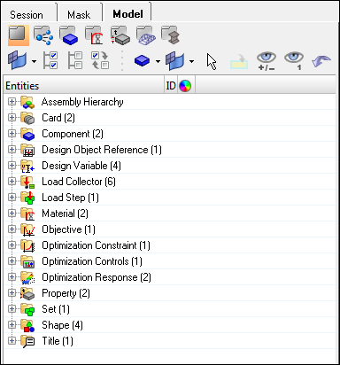
 to open the
Contour panel.
to open the
Contour panel.