Composite Stress Toolbox
Composite stress toolbox functionality.
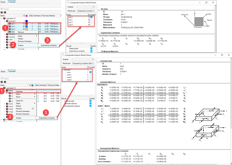
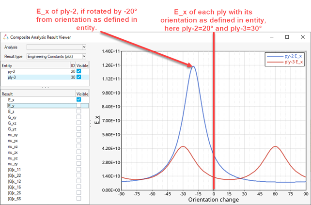
Composite stress toolbox functionality is provided in the Composite Browser. Engineering constants, load response, first ply failure, and strength analyses are included. All analyses are accessible via the Analysis entity driven workflow. Engineering constants are additionally accessible via the right-click context menu of relevant entities.
Engineering Constants
- Materials
- Plies
- Zones
- Laminates
- Elements
- Selection of multiple entities of the same type is also supported and generates a list in the Composite Analysis Result Viewer, from which desired results can be selected.
- Only one analysis entity can be selected and run at a given time. All analyses’ results can be accessed via the Analysis combo box in the Composite Analysis Result Viewer.
- Material data
- Engineering constants
- 2D/3D material matrices
- Strength allowables
- Thermal expansion coefficients
Calculations are output in the material system. Note that 3D properties can only be calculated for materials which provide the necessary data (for example, OptiStruct MAT9OR). Allowables are read from the materials basic data and additional MATF entries.
- Ply data
- Engineering constants
- 2D/3D material matrices
- Thermal expansion coefficients
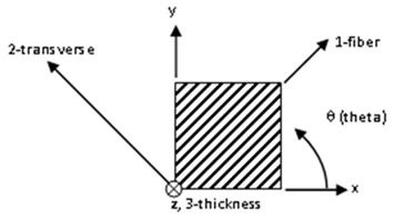
Calculations are output in the laminate’s material reference orientation. Accordingly, the ply angle entered in the ply Orientation field is used to transform the properties from ply fiber direction to the laminate material reference orientation. For more information, refer to Fiber Orientation.
- Laminate data
- Stiffness and compliance matrices
- Homogenized engineering constants
- Normalized homogenized matrices
- Thermal expansion coefficients
- Out-of-plane shear properties
- Laminate data
- Stiffness and compliance matrices
- Homogenized engineering constants
- Normalized homogenized matrices
- Thermal expansion coefficients
- Out-of-plane shear properties
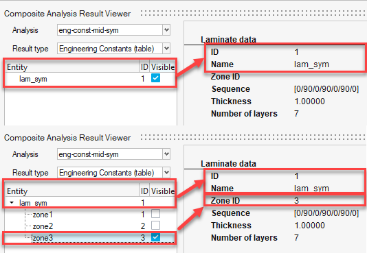
Additionally, stacking sequence, thickness and number of layers are summarized for each zone.
- Laminate data
- Stiffness and compliance matrices
- Homogenized engineering constants
- Normalized homogenized matrices
- Thermal expansion coefficients
- Out-of-plane shear properties
Additionally, stacking sequence, thickness, and number of layers are summarized for each zone. All properties are calculated assuming mid-plane laminates, hence offsets in properties are disregarded.
Engineering constants calculations are also available through the analysis entity driven workflow as outline in the following for other analysis types.
Load Response/Failure
The response of a laminate due to an applied load is calculated based on its behavior derived from Classical Laminate Theory. For transverse shear, First Order Shear Deformation Theory is used. Load response/failure analysis is run through an analysis entity with Type: Load response/failure. Mandatory analysis inputs are Entity (single or multi-selection of laminates or elements) and Plate load. The Plate load can be of type load, result subcases, or result simulations, where the latter 2 are only available with elements.
The Plate load type determines the solution sequence. For composite plate loads, no transformations are needed, as they are midplane loads and in a material coordinate system. For result subcases and result simulations, loads are read from the results files and transformed from an elemental system to a material system before being applied to the laminates on the elements. All results are calculated with respect to offsets provided on the property assigned to the element. This includes laminate properties used for the load response as well as the midplane results shown in the corresponding section.
The first ply failure (FPF) settings are optional and are used for first ply failure analysis.
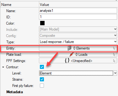
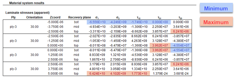
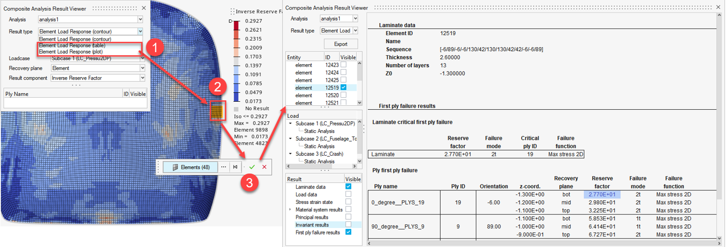
Table minimum and maximum values are indicated by blue and red cell background to quickly spot the extreme values of each result. For first ply failure calculation, the failure index is an exception. Here the failure index, which leads to the critical reserve factor, is marked red and the least critical is marked blue, see Figure 7.
- Laminate data
- Load data (in elemental and material coordinate system)
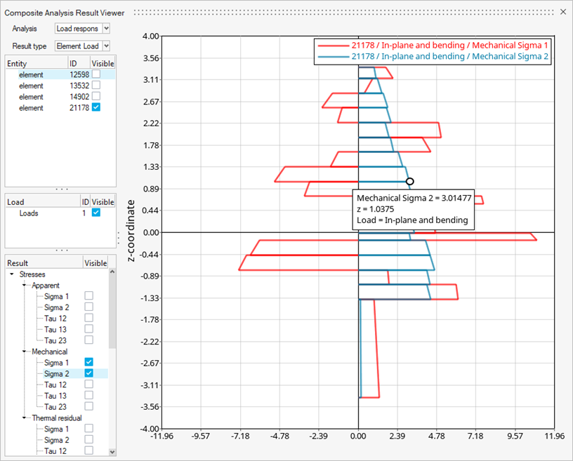
- Midplane loads (converted forces and moments, strains and curvatures, homogenized stresses)
- Material system stresses for each ply
- Apparent
- Mechanical
- Thermal residual
- Material system strains for each ply
- Apparent
- Mechanical
- Thermal
- Thermal free
- Thermal residual
- Principal stresses and strains for each ply
- Stress and strain invariants for each ply
- Optionally: First ply failure margins (in the form of reserve factor, margin of safety, inverse reserve factor, or failure index) for each ply, as well as laminate critical ply, failure mode and failure function
- Element mid-plane strains, first-ply-failure margins and critical ply ID
- Ply recovery planes’ (middle, top/bottom, top/middle/bottom) stresses and strains in corresponding ply material system, and first-ply-failure margins
Strength
Strength analysis calculates the failure loads for selected laminates for applying load components individually. Unit loads used for a load response/failure analysis and critical values are determined iteratively. Strength analysis is run through an analysis entity with Type: Strength. Mandatory analysis inputs are Entity (single or multi-selection of laminates) and FPF settings.
- Forces
- Moments
- Stresses (in-plane, flexural, out-of-plane)
- Strains (in-plane, flexural)
- Curvatures
- Failure mode and critical ply ID for each critical load
Composite Plate Loads
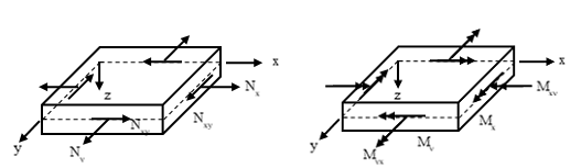
Composite stress toolbox utilizes 3 types of load vectors to calculate laminate load response. Each load vector consists of different load components. All composites plate loads are applied as midplane loads in the material system. The components are listed in the table below.
| Type | Components |
|---|---|
| Forces and moments | N_x, N_y, N_xy, M_x, M_y, M_xy, Q_x, Q_y, Delta T z_min, Delta T z_max |
| Strains and curvatures | Epsilon_x, Epsilon_y, Gammy_xy, Kappa_x, Kappa_y, Kappa_xy,
Delta T z_min, Delta T z_max Note: Strains
and curvatures are treated as initial strains and curvatures
when combined with thermal loads. |
| Homogenized stresses | Sigma_x, Sima_y, Tau_xy, Sigma^f_x, Sigma^f_y, Tau^f_xy, Tau_zx, Tau_yz, Delta T z_min, Delta T z_max |
Temperature differences with respect to laminate reference temperature can be defined for laminate top (z_max) and bottom (z_min) independently. The temperature distribution is assumed to be linear in between, also for laminates consisting of different materials.
First Ply Failure Methods
The First Ply Failure Method is a collection of mainly composite failure criteria, that can be utilized within the certification framework and the composite stress toolbox. The latter are applicable to Strength and Load response/failure analysis. They can be created from certification ribbon tools or directly from the right-click menu of the Composite Browser.
Workflow
To set up and run an analysis:
- Create and edit all participating entities (materials, plies, laminates, composite plate loads, first ply failure methods).
- Right-click in the white space of the Composite Browser or the Analyses folder to create an analysis entity.
- Select the analysis type.
- Select participating entities according to analysis type.
Figure 11. 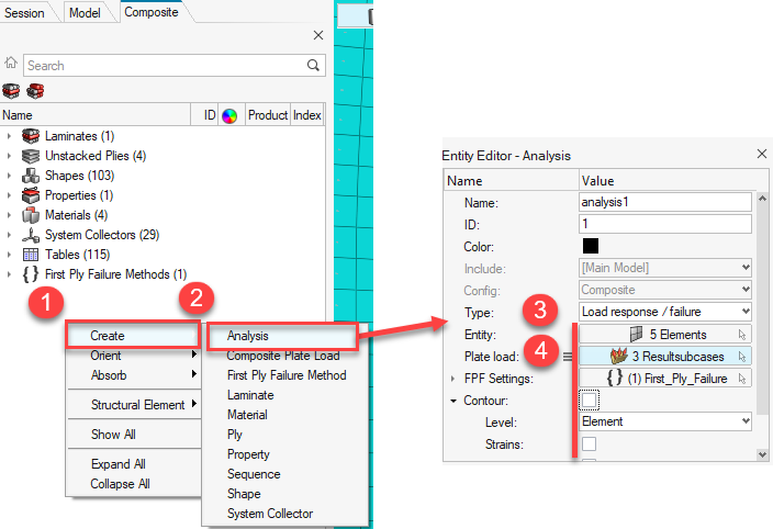
- Run using the analysis’ right-click menu option
Run….
In the result view, combinations of entities and results can be picked. When any of the participating entities are changed, the analysis must be run again.
- Export results from the Composite Analysis Result Viewer to
.csv file for numerical results and line data of
plots, as well as .png image file for the plots
themselves.Image files will be saved in the same size as displayed in the viewer at export time. Numerical (table) results from the Composite Analysis Result Viewer can be copied to the clipboard via the keyboard shortcut or via the context menu available in the result display area.
Figure 12. 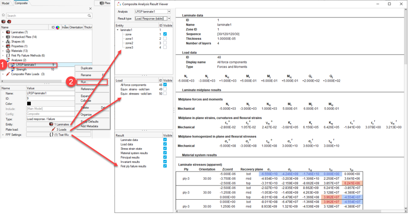
Solver Specific Details
Entities created in the Composite Browser are assigned the most common solver card for a typical ply-based model. Properties and Shapes are filtered based on solver card to only display appropriate cards for a ply-based model. Additionally, in the OptiStruct profile, the appropriate card is set for laminate and ply entities upon creation.
| Entity | Supported Cards |
|---|---|
| Laminate | STACK |
| Material | MAT1, MAT2, MAT8, MAT9OR, MATMDS, MATF |
| Ply | PLY |
| Zone | None |
| Result file type | *.op2, *.h3d, *.h5, *.hdf5 |
| Entity | Supported Cards |
|---|---|
| Laminate | Via property *SHELL_SECTION_COMPOSITE |
| Material | *MATERIAL, with type ISOTROPIC, ENGINEERING CONSTANTS, LAMINA, or USER MATERIAL |
| Ply | None |
| Zone | None |
| Entity | Supported Cards |
|---|---|
| Laminate | Via property PCOMPP realized to PCOMP or PCOMPG |
| Material | MAT1, MAT2, MAT8, MATORT |
| Ply | None |
| Zone | None |
| Result file type | *.xdb |
- OptiStruct: PCOMP(G), PCOMPP, PSHELL (MAT1, MAT2, MAT8)
- Nastran: PCOMP(G), PSHELL (MAT1, MAT2, MAT8)
- Abaqus: SHELLSECTION_COMPOSITE
Element offsets are considered for load response calculations by using the ZOFFS values for PCOMP(G) and PCOMPP properties in OptiStruct and Nastran. For PSHELL with MAT1 or MAT8 material (MID1) assignment, the value of ZOFFS is also used and the analysis is run using MID1 material to compute in-plane, bending and transverse shear properties. Other MID (2,3,4) assignments are disregarded. For PSHELL with MAT2 assigned, MID4 can be used to introduce coupling effects. MID4 data is incorporated into the classical laminate theory calculations, while indicating Z0=-0.5 (mid-plane) in the laminate data, as the actual offset is unknown. PSHELL is treated as a single layer for all analysis types.