HS-1080: Set Up an Operator Model

Learn how to use the Operator model type to run a script that uses a combination of HyperView and HVTrans to split the solver result file in multiple result files, one for each component in the model.

Before you begin, copy the model files used in this tutorial from <hst.zip>/HS-1080/ to your working directory.

This tutorial uses a model which consists of a plate with a hole which is loaded in plane. The design has three thickness variables; one for each zone. The output responses of interest are the maximum stress in each of the three zones.

Perform the Study Setup

  1. Start HyperStudy.
  2. Start a new study in the following ways:
    • From the menu bar, click File > New.
    • On the ribbon, click .
  3. In the Add Study dialog, enter a study name, select a location for the study, and click OK.
  4. Go to the Define Models step.
  5. Add a Parameterized File model.
    1. From the Directory, drag-and-drop the plate.tpl file into the work area.
      Figure 1.


    2. In the Solver Input File column, enter plate.fem.
      This is the name of the solver input file HyperStudy writes during any evaluation.
    3. In the Solver Execution Script column, select OptiStruct (os).
    Figure 2.


  6. Click Import Variables.
    Three input variables are imported from the plate.tpl resource file.
  7. Go to the Define Input Variables step.
  8. Review the input variable's lower and upper bound ranges.

Perform Nominal Run

  1. Go to the Test Models step.
  2. Click Run Definition.
    An approaches/setup_1-def/ directory is created inside the study Directory. The approaches/setup_1-def/run__00001/m_1 directory contains the input file, which is the result of the nominal run.

Set Up the Operator Model

You cannot set up the operator model until after the nominal run is complete and the plate.h3d file has been generated.
  1. Go to the Define Models step.
  2. Add an Operator model.
    1. Click Add Model.
    2. In the Add - HyperStudy dialog, select Operator and click OK.
  3. Click Model Resources.
    The Model Resources dialog opens.
  4. Define a model dependency that references the python script that will be used as the solver script.
    This is a reference to a file that is not generated during a solver run, therefore it is of type Normal. This file does not need to be in the run directory.
    1. Select Operator 1 (m_2).
    2. Click Resource Assistant > Add File.
    3. In the Select File dialog, navigate to your working directory and open the corresponding file:
      Table 1.
      Option Description Location Operation
      Python based model

      hv_resultsbyComp.py

      hv_resultsbyComp.tcl

      plate.h3d

      Study directory

      Study directory

      m_1 folder

      None

      Copy

      Copy

      Direct Solver (hw.exe) Model

      hv_resultsbyComp.tcl

      plate.h3d

      Study directory

      m_1 folder

      None

      Copy

      Figure 3. Model Resources for Python Model
      Figure 4. Model Resources for HyperWorks Model
  5. Set the Solver execution script.
    OptionDescription
    Python based model
    1. Set the Solver Execution Script to Python (py).
    2. In the Solver Input Arguments column, enter ${m_2.file_2} ${m_2.file_4}.

    The input arguments are references to the model resources' varnames. The first argument (m_2.file_2) is a reference to the model resource’s varname, and tells python which script to run. The second argument (m_2.file_4) is the varname to the target result file to split, and will be the first argument to the python script.

    Figure 5.
    Direct Solver (hw.exe) Model
    1. Set the Solver Execution Script to HyperWorks (hw.exe).
    2. In the Solver Input Arguments column, enter -tcl ${m_2.file_2} -b -result ${m_2.file_3}.

    The input arguments are references to the model resources' varnames. The first argument (m_2.file_2) is a reference to the model resource’s varname, and tells hw.exe which tcl script to run. The second argument (m_2.file_3) is the varname to the target result file to split.

    Figure 6.

Perform Nominal Run

  1. Go to the Test Models step.
  2. Click Run Definition.
  3. In the Altair HyperStudy dialog, click Overwrite.
    The m_1 and m_2 directories are created inside the approaches/setup_1-def/run__00001/ directory.

Create and Evaluate Output Responses

In this step you will create four output responses: maxStressPart2, maxStressPart4, maxStress3, Volume.

  1. Go to the Define Output Responses step.
  2. Create the maxStressPart2 output response.
    1. From the Directory, drag-and-drop the plate_2_shell.h3d file, approaches/setup_1-def/run__00001/m_2, into the work area.
    2. In the File Assistant dialog, set the Reading Technology to Altair® HyperWorks® (Hyper3D Reader) and click Next.
    3. Select Multiple Items at Multiple Time Steps, then click Next.
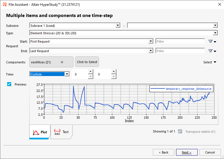
    4. Define the following options, and then click Next.
      • Set Subcase to Subcase 1(Load).
      • Set Type to Element Stresses (2D & 3D) (2D).
      • For Request, set Start to First Request and End to Last Request.
      • For Components, select vonMises (Z1).
      • For Time, select Custom and enter 0.
      Figure 7.


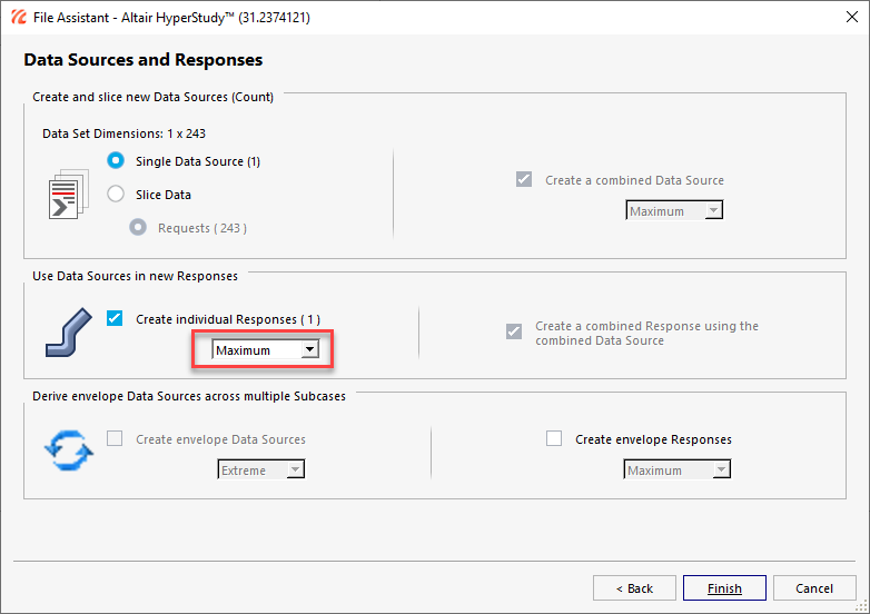
    5. Under Use Data Source in new Responses, select Maximum.
      Figure 8.


    6. Click Finish.
      The output response is displayed in the work area.
    7. In the Label field, enter maxStressPart2.
      Figure 9.


  3. Create the maxStressPart4 output response.
    1. From the Directory, drag-and-drop the plate_4_patch2.h3d file, located in approaches/setup_1-def/run__00001/m_2, into the work area.
    2. In the File Assistant dialog, set the Reading technology to Altair® HyperWorks® (Hyper3D Reader) and click Next.
    3. Select Multiple Items at Multiple Time Steps, then click Next.
    4. Define the following options, and then click Next.
      • Set Subcase to Subcase 1(Load).
      • Set Type to Element Stresses (2D & 3D) (2D).
      • For Request, set Start to First Request and End to Last Request.
      • For Components, select vonMises (Z1).
      • For Time, select Custom and enter 0.
    5. Under Use Data Source in new Responses, select Maximum.
    6. Click Finish.
      The output response is added to the work area.
    7. In the Label field, enter maxStressPart4.
  4. Create the maxStress3 output response.
    1. From the Directory, drag-and-drop the plate_3_patch1.h3d file, located in approaches/setup_1-def/run__00001/m_2, into the work area.
    2. In the File Assistant dialog, set the Reading technology to Altair® HyperWorks® (Hyper3D Reader) and click Next.
    3. Select Multiple Items at Multiple Time Steps, then click Next.
    4. Define the following options, and then click Next.
      • Set Subcase to Subcase 1(Load).
      • Set Type to Element Stresses (2D & 3D) (2D).
      • For Request, set Start to First Request and End to Last Request.
      • For Components, select vonMises (Z1) and vonMises (Z2).
      • For Time, select Custom and enter 0.
    5. Under Use Data Source in new Responses, select Maximum.
    6. Click Finish.
      The output response is added to the work area.
    7. In the Label field, enter maxStress3.
  5. Create the Volume output response.
    1. From the Directory, drag-and-drop the plate.out file, located in approaches/setup_1-def/run__00001/m_1, into the work area.
    2. In the File Assistant dialog, set the Reading technology to Altair® HyperWorks® (osmass.tpl) and click Next.
    3. Select Single Item in a Time Series, then click Next.
    4. Define the following options, and then click Next.
      • Set Type to OptiStruct Analysis.
      • Set Request to Out File.
      • Set Component to Volume.
    5. Label the output response Volume.
    6. Set Expression to Maximum.
    7. Click Finish.
    The Volume output response is added to the work area.
  6. Click Evaluate to extract the response values.
Figure 10.


Run DOE

  1. Add a DOE.
    1. In the Explorer, right-click and select Add from the context menu.
      The Add dialog opens.
    2. From Select Type, choose DOE.
    3. For Definition from, select an approach.
    4. Select Setup and click OK.
  2. Go to the DOE 1 > Specifications step.
  3. In the work area, set the Mode to Modified Extensible Lattice Sequence.
  4. Click Apply.
  5. Go to the DOE 1 > Evaluate step.
  6. Click Evaluate Tasks.
  7. Go to the DOE 1 > Post-Processing step.
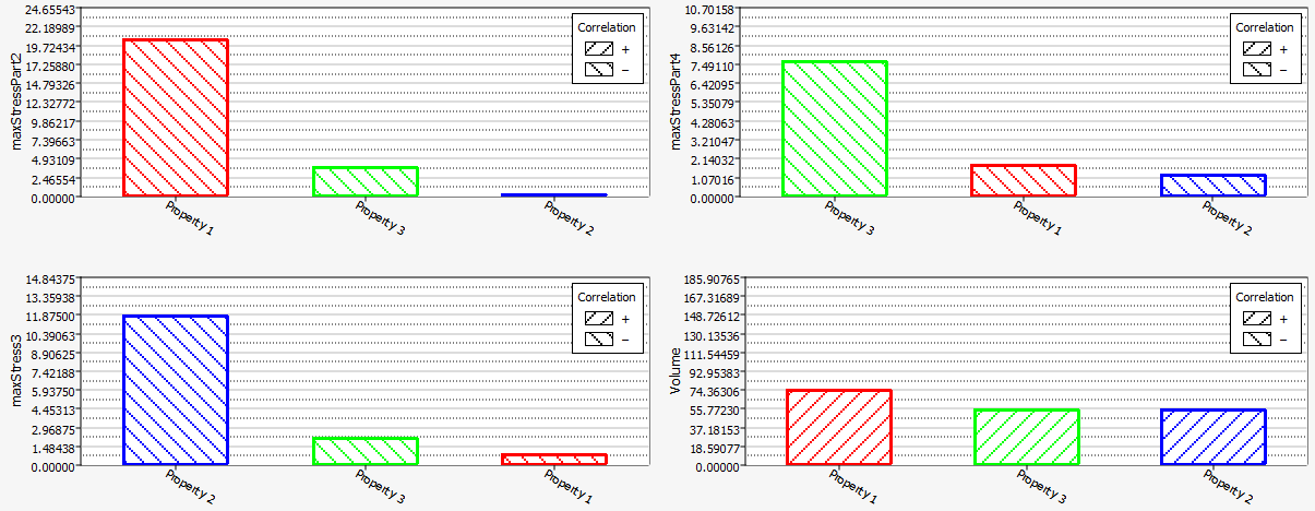
  8. Click the Pareto Plot tab to plot the effects of variables on output responses in hierarchical order (highest to lowest).
    Each variable contributes nearly equally to volume. A positive hashing indicates that the relationship is positive: as the variable increases, mass increases. For the three stress output responses, the maximum stress in each zone is dominated by the thickness of that zone.
    Figure 11.