Tutorial Level: Beginner Learn how to set up a study on simple functions defined using an Internal Math
model.
In this tutorial you will set up a beverage can design of experiments to see how
design variables effect the responses. The beverage has the following design
variables and output responses:
Design variables
Diameter
Height
Output responses
Material Cost
Volume
Perform the Study Setup
Start HyperStudy.
Start a new study in the following ways:
From the menu bar, click File > New.
On the ribbon, click .
In the Add Study dialog, enter a study name, select a
location for the study, and click OK.
Go to the Define Models step.
Add an Internal Math model.
Click Add Model.
In the Add dialog, select Internal
Math and click OK.
Go to the Define Input Variables step.
Create two input variables.
Click Add Input Variables twice.
In the work area, Label column, change the labels for the two input
variables to Diameter and
Height.
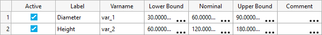
Change both input variable's lower, nominal, and upper bounds to the
values indicated in Figure 1.
Figure 1.
Perform Nominal Run
Go to the Test Models step.
Click Run Definition.
An approaches/setup_1-def/ directory is created
inside the Study Directory. The
approaches/setup_1-def/run__00001/m_1 directory
contains the input file, which is the result of the nominal run.
Create and Evaluate Output Responses
In this step you will create the output responses, Cost and Volume.
Go to the Define Output Responses step.
Create two output responses.
Click Add Output Responses two times.
In the work area, Label column, change the labels for the output
responses to Cost and
Volume.
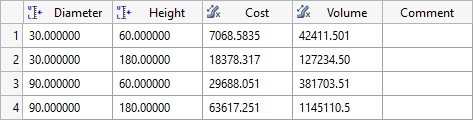
In the Expression column, enter the following:
For Cost, enter
2*(pi*var_1^2/4)+var_2*pi*var_1.
For volume, enter (pi*var_1^2/4)*var_2.
Figure 2.
Click Evaluate to extract the response values.
Run DOE
Add a DOE.
In the Study Explorer, right-click and select
Add from the context menu.
The Add dialog opens.
From Select Type, choose
DOE.
For Definition from, select an approach.
Select Setup and click OK.
Go to the DOE 1 > Specifications step.
In the work area, set the Mode to Full
Factorial.
Click Show more... to expand the selection
window.
Click Apply.
Go to the DOE 1 > Evaluate step.
Click Evaluate Tasks.
Go to the DOE 1 > Post-Processing step.
Click the Summary tab.
There are two input variables with lower and upper bounds which result in 22 =
4 runs.Figure 3.
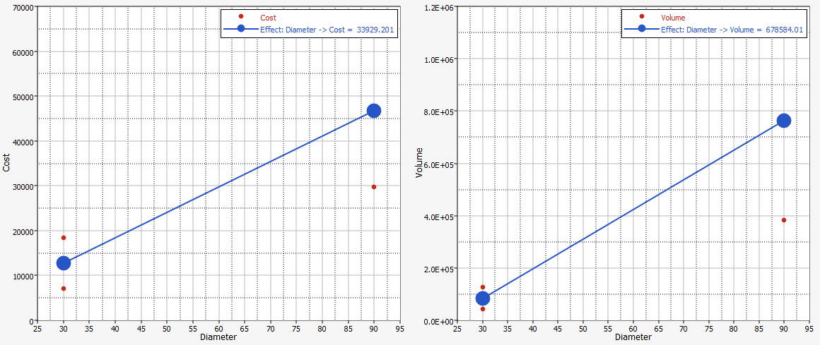
Click the Linear Effects tab.
The data collected in the Summary tab is used to calculate the linear effects
of the Diameter and Height input variables on the Cost and Volume output
responses. A line is drawn between the average value of the output response when
the input variable is at its lower bound and the average value of the output
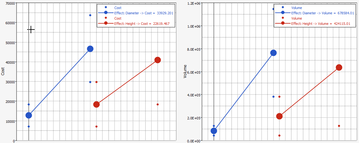
response when the input variable is at its upper bound.Figure 4. Effects Computation of Diameter on Cost and Volume The effects of the input variable Height on the output responses Cost and
Volume are computed in the same manner. By displaying both input variables and
output responses in the same plot, you can compare the effects.
Note: Ctrl+Click allows you to select more than one
variable/response.
Figure 5. The slope of the lines could be positive or negative. In this example,
both effects have a positive slope which indicates that increasing the input
variable's values will also increase the output responses.

 .
.