AcuSolve Enclosure Radiation

Enclosure Radiation Methodology

AcuSolve simulates the surface to surface radiation using a two step approach:

View factor computation: In radiative heat transfer view factor is the proportion of radiation incident on one surface due to another surface. The view factors for each facet defining the radiation enclosure are computed using the hemicube algorithm and smoothed using least squares method as a pre-processing step. The view factors are not recomputed during the simulation.
Heat flux addition: The radiative heat flux, based on view factors, computed using the Stefan-Boltzmann law and the total radiosity, based on Kirchoff's law, is added to the enthalpy transport equation during the solver run.

The enclosure radiation model is supported only on fluid mediums, that is, the fluid side of the fluid/solid surface.

View factor computation is an important point when dealing with moving mesh simulation. Since the view factors are not recomputed during the solver run the boundary elements forming the enclosure should not deform.

The total emissive power of a grey surface is given by the Stefan-Boltzmann law:

W_{i} = ϵ_{i} σ {(T_{i} + T_{o f f})}^{4}

where $ϵ_{i}$ is the emissivity of surface i, given by an EMISSIVITY_MODEL command; $σ$ is the Stefan-Boltzmann constant, given by stefan_boltzmann_constant; T_i is the temperature of surface i; and T_off is the offset to convert to an absolute temperature, given by the absolute_temperature_offset parameter of the EQUATION command. In addition, each surface receives part of the total radiosity from each of the radiation surfaces:

G_{i} = \sum_{j}^{} F_{i j} J_{j}

where G_i is the total irradiation of the surface i, F_ij is the view factor from the surface i to surface j and J_j is the total radiosity from surface j. The total radiosity of surface i is

J_{i} = W_{i} + (1 - α_{i}) G_{i}

where $α_{i}$ is the absorptivity and $1 - α_{i}$ is the reflectivity. From Kirchhoff' law and the grey surface assumption, $α = ϵ$ . The net radiation heat flux is thus $q_{i} = G_{i} - J_{i} = α_{i} G_{i} - W_{i}$ and is added to the temperature equation. The radiation equation solves for all the radiation heat fluxes coupled together with the temperature equation.

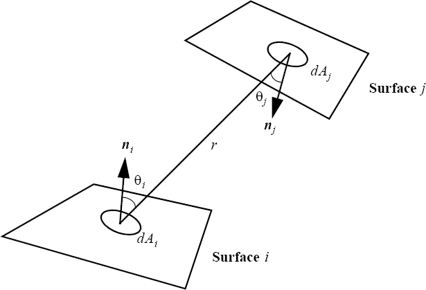
View factors $F_{i j}$ are purely geometric entities defined as

F_{i j} = \frac{1}{A_{i}} \int_{A_{i}}^{} \int_{A_{j}}^{} \frac{\cos θ_{i} \cos θ_{j}}{π r^{2}} δ_{i j} d A_{i} d A_{j}

where A_i and A_j are the areas of surfaces i and j, respectively; $θ_{i}$ and $θ_{j}$ are the angles between the line connecting $d A_{i}$ to $d A_{j}$ and the normals to surfaces $d A_{i}$ to $d A_{j}$ ; respectively; r is the distance from $d A_{i}$ to $d A_{j}$ ; and $δ_{i j}$ is the visibility function, it is equal to one if $d A_{i}$ to $d A_{j}$ see each other, otherwise it is zero.

View Factor Nomenclature

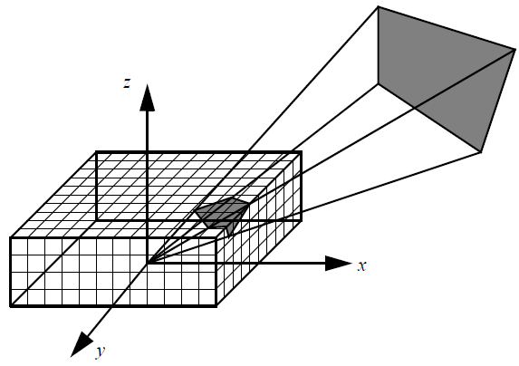
The view factors are computed using the hemicube algorithm. In a nutshell, in this algorithm a hemicube is placed on the centroid of each radiation facet i. The hemicube is discretized into 3n² pixels; where n is given by num_hemicube_bins. All surfaces (facing surface i) are then projected onto this hemicube. The Z-buffering algorithm is used to compute the visibility. Once all surfaces are projected, the pixels weighted by their view factor increments are added up to determine a row of F_i={F_ij}.

Hemicube Discretization

The hemicube algorithm has three major assumptions, and hence sources of errors: aliasing - the true projection of each visible face onto the hemicube can be accurately accounted for by using a finite resolution hemicube; proximity - the distance between faces is great compared to the effective diameter of the faces; and visibility - the visibility between any two faces does not depend on the position within either face. The aliasing error may be reduced through the use of larger num_hemicube_bins values, at the expense of computational cost. The computational cost is proportional to n² for sufficiently large values of n. In addition, a random jittering algorithm and a non-uniform hemicube pixelization are employed to minimize the aliasing error. The proximity and visibility errors occur when two facing facets are too close to each other. In this case, the geometry of one or both facets cannot be sufficiently well-represented by their centroids. These errors can be reduced by splitting each poorly-represented facet into smaller segments (sub-surfaces), computing the view factors separately for each sub-surface and then adding them up. The computational cost is proportional to the number of sub-surface divisions. The max_surface_subdivision parameter may be used to trade-off accuracy against cost.

A least-squares smoothing is automatically applied to the computed view factor matrix to enforce reciprocity and conservation:

$A_{i} F_{i j} = A_{j} F_{j i}$ (reciprocity)

$\sum_{j}^{} F_{i j} = 1$ (conservation)

Note: Due to the cost of computing the view factor matrix, it is computed in a pre-processing step and stored on disk. This means that the view factors are not updated during a simulation, even when mesh movement is present.

The default for the Stefan-Boltzmann constant is given in MKS units: $σ = 5.670 \times 10^{- 8} W / (m^{2} ° K^{4})$ .

In British units it is: $σ = 4.756 \times 10^{- 11} B t u / (s f t^{2} ° R^{4})$ .

In general, this constant must be converted to be consistent with the units chosen for use in the problem.