
MESH_MOTION
Specifies mesh motion of nodes.
Type
AcuSolve Command
Syntax
MESH_MOTION("name") {parameters...}
Qualifier
User-given name.
Parameters
- type (enumerated) [=none]
- Mesh motion type.
- none
- No boundary conditions imposed.
- zero
- Nodes fixed in space.
- translation
- Simple linear translation.
- rotation
- Simple rotation.
- piecewise_linear or linear
- Motion computed from piecewise linear curve fit of two points.
- cubic_spline or spline
- Motion computed from cubic spline curve fit of two points.
- user_function or user
- Motion described by a user function.
- rigid_body_dynamic or rigid
- Nodes move dynamically as a rigid body.
- interpolated_motion
- Nodes move based on the motion of interpolated motion surfaces. Requires interpolated_motion_surfaces.
- translation_velocity or vel (array) [={0,0,0}]
- Translation velocity. Used with translation type.
- translation_variable (enumerated) [=time]
- Scaling of translation velocity to obtain translation. Used with
translation type.
- time
- Time.
- multiplier_function
- The multiplier function for the temporal function of the translation. Requires translation_variable_multiplier_function.
- multiplier_function_on_time
- The multiplier function for the temporal function of the translation velocity for computing the translation by time integration of translation velocity. Requires translation_variable_multiplier_function.
- translation_variable_multiplier_function (string) [=none]
- User-given name of the multiplier function for computing the translation. If none, the translation is zero. Used with multiplier_function translation variable.
- rotation_center (array) [={0,0,0}]
- Center of rotation, specified in global xyz coordinate system. Used with rotation type.
- angular_velocity or ang_vel (array) [={0,0,0}]
- Angular velocity, in radians per unit of time. Used with rotation type.
- rotation_variable (enumerated) [=time]
- Scaling of angular velocity to obtain the rotation angle. Used with
rotation type.
- time
- Time.
- multiplier_function
- The multiplier function for the temporal function of the rotation angle. Requires rotation_variable_multiplier_function.
- multiplier_function_on_time
- The multiplier function for the temporal function of the angular velocity for computing the rotation angle by time integration of angular velocity. Requires rotation_variable_multiplier_function.
- rotation_variable_multiplier_function (string) [=none]
- User-given name of the multiplier function for computing the rotation angle. If none, the rotation is zero. Used with multiplier_function rotation variable.
- curve_fit_values or curve_values (array) [={0,0,0,0,1,0,0}]
- Data for the motion of two points as a function of an independent variable. Used with piecewise_linear or cubic_spline type. Requires curve_fit_variable.
- curve_fit_variable or curve_var (enumerated) [=time]
- Independent variable for the mesh motion data. Used with
piecewise_linear or cubic_spline type.
- time
- Time.
- multiplier_function
- Multiplier function. Requires curve_fit_variable_multiplier_function.
- curve_fit_variable_multiplier_function or curve_name (string) [=none]
- User-given name of the multiplier function that represents the independent variable of the curve fit for computing the mesh motion. If none, the motion is zero. Used with multiplier_function curve fit variable.
- user_function or user (string) [no default]
- Name of the user-defined function. Used with user_function type.
- user_values (array) [={}]
- Array of values to be passed to the user-defined function. Used with user_function type.
- user_strings (list) [={}]
- Array of strings to be passed to the user-defined function. Used with user_function type.
- interpolated_motion_surfaces (list) [={}]
- List of surfaces whose motions are used to scale the displacements of mesh nodes in between. Each surface is defined by one instance of the INTERPOLATED_MOTION_SURFACE command.
- rigid_body_x_displacement (enumerated) [=active]
- Constraint on x displacement of rigid body. Used with rigid_body type.
- active
- No constraint.
- Zero
- Zero x displacement.
- rigid_body_y_displacement (enumerated) [=active]
- Constraint on y displacement of rigid body. Used with rigid_body type.
- active
- No constraint.
- Zero
- Zero y displacement.
- rigid_body_z_displacement (enumerated) [=active]
- Constraint on z displacement of rigid body. Used with rigid_body type.
- active
- No constraint.
- Zero
- Zero z displacement.
- rigid_body_x_rotation (enumerated) [=active]
- Constraint on rotation around x axis of rigid body. Used with rigid_body type.
- active
- No constraint.
- Zero
- Zero x axis rotation.
- rigid_body_y_rotation (enumerated) [=active]
- Constraint on rotation around y axis of rigid body. Used with rigid_body type.
- active
- No constraint.
- Zero
- Zero y axis rotation.
- rigid_body_z_rotation (enumerated) [=active]
- Constraint on rotation around z axis of rigid body. Used with rigid_body type.
- active
- No constraint.
- Zero
- Zero z axis rotation.
- rigid_body_rotation_only (boolean) [=off]
- Activated when the rigid body motion is fixed-point rotation and type is set to rigid_body_dynamic. Used with rigid_body_center, rigid_body_external_force and rigid_body_moment_arm.
- rigid_body_center (array) [={0,0,0}]
- Used with type = rigid_body_dynamic and specified in the global xyz coordinate system, rigid_body_center denotes the origin of the local xyz coordinate system. When the rigid body is doing general three-dimensional motion with both translation of center of mass and rotation around center of mass, rigid_body_center should be the coordinates of center of mass at time=0. When rigid_body_rotation_only = on (the rigid body is doing fixed-point rotation) rigid_body_center is regarded as the fixed rotation center, not necessarily center of mass. Notice that the effect of gravity or other external force, whenever needed, can be taken into account by using rigid_body_external force and rigid_body_moment_arm.
- rigid_body_moment_arm (array) [={0,0,0}]
- Used when rigid_body_rotation_only = on. The coordinate, specified in the local xyz coordinate system, of the location of the concentrated external force, specified by rigid_body_external_force. In the case of gravity, it is the center of mass specified in the local coordinate system.
- rigid_body_direction (array) [={1,0,0;0,1,0;0,0,1}]
- Direction of local xyz coordinate system, specified with respect to the global xyz coordinate system. First row is the local x direction. Used with rigid_body type.
- rigid_body_mass (real) >0 [=1]
- Mass of the rigid body. Used with rigid_body type.
- rigid_body_dyadic (array) [={1,1,1,0,0,0}]
- Symmetric dyadic (moment of inertia] matrix for the rotational rigid body equation. Used with rigid_body type.
- rigid_body_stiffness (array) [={0,0,0,0,0,0}]
- Symmetric stiffness matrix for the translational rigid body equation. Used with rigid_body type.
- rigid_body_damping (array) [={0,0,0,0,0,0}]
- Symmetric damping matrix for the translational rigid body equation. Used with rigid_body type.
- rigid_body_rotational_stiffness (array) [={0,0,0,0,0,0}]
- Symmetric rotational stiffness matrix for the rotational rigid body equation. If this parameter is non-zero, rotations are limited to π radians. Used with rigid_body type.
- rigid_body_rotational_damping (array) [={0,0,0,0,0,0}]
- Symmetric rotational damping matrix for the rotational rigid body equation. Used with rigid_body_dynamic type.
- rigid_body_external_force_type (enumerated) [constant]
- Type of rigid body external force. Used with rigid_body_dynamic
type.
- constant
- External force vector components are constant values.
- piecewise_linear or linear
- External force vector components are linear functions of time.
- cubic_spline or spline
- External force vector components are cubic functions of time.
- user_function or user
- External force vector components are provided by user function.
- rigid_body_external_force (array) [={0,0,0}]
- External force vector on rigid body, specified in the global coordinate system. Used with rigid_body_external_force_type = constant.
- rigid_body_external_force_curve_fit_values (array) [={0,0,0,0}]
- A four column array of independent-variable/force data values. Used with rigid_body_external_force_type = piecewise_linear or cubic_spline.
- rigid_body_external_force_curve_fit_variable (enumerated) [=time]
- Independent-variable of the curve fit. Used with
rigid_body_external_force_type =
piecewise_linear or cubic_spline.
- time
- Physical time.
- rigid_body_external_force_user_function (string) [no default]
- Name of the user-defined function. Used with rigid_body_external_force_type = user_function.
- rigid_body_external_force_user_values (array)[={}]
- Array of values to be passed to the user-defined function. rigid_body_external_force_type = user_function.
- rigid_body_external_force_user_strings (list)[=none]
- Array of strings to be passed to the user-defined function. rigid_body_external_force_type = user_function.
- rigid_body_external_force_multiplier_function (string) [=none]
- User-given name of the multiplier function for scaling the external force. If none, no scaling is performed. Used with rigid_body_dynamic type.
- rigid_body_external_moment_type (enumerated) [constant]
- Type of rigid body external moment. Used with
rigid_body_dynamic type.
- constant
- External moment vector components are constant values.
- piecewise_linear or linear
- External moment vector components are linear functions of time.
- cubic_spline or spline
- External moment vector components are cubic functions of time.
- user_function or user
- External moment vector components are provided by user function.
- rigid_body_external_moment (array) [={0,0,0}]
- External moment vector on rigid body. Used with rigid_body_external_moment_type = constant.
- rigid_body_external_moment_curve_fit_values (array) [={0,0,0,0}]
- A four column (array) of independent-variable/moment data values. Used with rigid_body_external_moment_type = piecewise_linear or cubic_spline.
- rigid_body_external_moment_curve_fit_variable (enumerated) [=time]
- Independent-variable of the curve fit. Used with
rigid_body_external_moment_type =
piecewise_linear or cubic_spline.
- time
- Physical time.
- rigid_body_external_moment_user_function (string) [no default]
- Name of the user-defined function. Used with rigid_body_external_moment_type = user_function.
- rigid_body_external_moment_user_values (array) [={}]
- Array of values to be passed to the user-defined function. Used with rigid_body_external_moment_type = user_function.
- rigid_body_external_moment_user_strings (list) [=none]
- Array of strings to be passed to the user-defined function. Used with rigid_body_external_moment_type = user_function.
- rigid_body_external_moment_multiplier_function (string) [=none]
- User-given name of the multiplier function for scaling the external moment. If none, no scaling is performed. Used with rigid_body_dynamic type.
- rigid_body_initial_displacement (array) [={0,0,0}]
- Initial displacement vector of the rigid body. Used with rigid_body_dynamic type.
- rigid_body_initial_velocity (array) [={0,0,0}]
- Initial velocity vector of the rigid body. Used with rigid_body_dynamic type.
- rigid_body_initial_rotation (array) [={0,0,0}]
- Initial rotation vector of the rigid body. Used with rigid_body_dynamic type.
- rigid_body_initial_angular_velocity (array) [={0,0,0}]
- Initial angular velocity vector of the rigid body. Used with rigid_body_dynamic type.
- rigid_body_initial_force (array) [={0,0,0}]
- Initial internal force vector on the rigid body. Used with rigid_body_dynamic type.
- rigid_body_internal_force_multiplier_function (string) [=none]
- User-given name of the multiplier function for scaling the internal force. If none, no scaling is performed. Used with rigid_body_dynamic type.
- rigid_body_initial_moment (array) [={0,0,0}]
- Initial internal moment vector on the rigid body. Used with rigid_body_dynamic type.
- rigid_body_internal_moment_multiplier_function (string) [=none]
- User-given name of the multiplier function for scaling the internal moment. If none, no scaling is performed. Used with rigid_body_dynamic type.
- rigid_body_filter (enumerated) [=none]
- Type of filter to smooth the internal forces and moments. Used with
rigid_body_dynamic type.
- none
- No filter.
- iir
- Infinite impulse response digital filter. Requires rigid_body_iir_input_coefficients and rigid_body_iir_output_coefficients.
- rigid_body_iir_input_coefficients (array) [={1}]
- Infinite impulse response digital filter coefficients applied to computed values. Used with iir rigid body filter and rigid_body_dynamic type.
- rigid_body_iir_output_coefficients (array) [={}]
- Infinite impulse response digital filter coefficients applied to previously filtered values. Used with iir rigid body filter and rigid_body_dynamic type.
- rigid_body_surface_outputs (list) [={}]
- Array of SURFACE_OUTPUT command qualifiers used to calculate the force and moment on the rigid body. Used with rigid_body_dynamic type.
Description
This command is used to simplify the specification of boundary conditions on mesh displacement, and in some cases to eliminate the solution of a hyperelastic equation normally needed to move the mesh nodes. In addition it can be used to simulate the dynamic motion of a rigid body.
MESH_MOTION( "rotating fan" ) {
   type                                = rotation
   rotation_variable                   = time
   rotation_center                     = { 0, 0, 0 }
   angular_velocity                    = { 0, 3, 0 }
}
ELEMENT_SET( "rotating fan" ) {
   mesh_motion                         = "rotating fan"
   ...
}
EQUATION {
   mesh                                = specified
   ...
}
In this example, the frame of reference does not rotate, as opposed to the first example in REFERENCE_FRAME, but instead all the mesh nodes in the element set rotate around the y axis at the rate of three radians per unit of time with the axis of rotation centered at the point (zero, zero, zero) in the global xyz coordinate system. The right hand rule is used to define the direction of rotation of the nodes. For this example, the location of each node in the element set is given by
MESH_MOTION( "Washing Machine" ) {
    type                                         = rotation
    rotation_variable                            = multiplier_function
    rotation_variable_multiplier_function        = "Washing Machine"
    rotation_center                              = { 0, 0, 0 }
    angular_velocity                             = { 0, 1, 0 }
}
MULTIPLIER_FUNCTION( "Washing Machine" ) {
    type                                         = piecewise_linear
    curve_fit_values                             = {    0, 0 ;
                                                      0.5, -10*PI/180 ;
                                                      1.0, 0 ;
                                                      1.5, +10*PI/180 ;
                                                      2.0, 0 ;
                                                      }
   curve_fit_variable                            = cyclic_time
   curve_fit_variable_cyclic_period              = 2
}MULTIPLIER_FUNCTION( "Washing Machine" ) {
type = piecewise_linear
curve_fit_values = { 0, 0 ;
0.5, -30*PI/180 ;
1.0, 0 ;
1.5, +30*PI/180 ;
2.0, 0 ;
}
curve_fit_variable = cyclic_time
curve_fit_variable_cyclic_period = 2
}MESH_MOTION( "moving train" ) {
type = translation
translation_variable = time
translation_variable_multiplier_function = "none"
translation_velocity = { 1, 0, 0 }
}
ELEMENT_SET( "train" ) {
mesh_motion = "moving train"
...
}Here all the nodes of the element set move at a constant velocity of one in the positive x direction. For this case, the location of each node in the element set is given by
where fn is the initial location of the node, v is given by translation_velocity, and t is time. Analogous to the rotation case, a multiplier function can be defined with translation_variable=multiplier_function to modify the scaling of velocity. Then the location of each node is given by
where f is given by translation_variable_multiplier_function.
A mesh motion type of none has the same effect as not referencing the MESH_MOTION command at all. This parameter is useful, for example, when you want to define a mesh motion but not activate it until a restart. A mesh motion type of zero is equivalent to specifying a NODAL_BOUNDARY_CONDITION command with type zero for each of the three components of mesh displacement.
MESH_MOTION( "general motion" ) {
   type                                          = piecewise_linear
   curve_fit_values                              = { 0, 0, 0, 0, 1, 0, 0 ; 1, 1, 0, 0, 0, 1, 0 ; }
   curve_fit_variable                            = time
   curve_fit_variable_multiplier_function        = "none"
}
This command will create a combined translation and rotation motion whereby the point originally at the origin is moved in the x direction and a point originally one unit along the x axis is moved along the y axis. As with the translation and rotation types, the time variable can be replaced with a multiplier function by specifying multiplier_function for curve_fit_variable and the name of a multiplier function for curve_fit_variable_multiplier_function.
A mesh motion type of user_function may be used to model more complex behaviors; see the AcuSolve User- Defined Functions Manual for a detailed description of user-defined functions. Unlike the curve fit types above, the user-defined function returns a 3x4 matrix that describes the combined translation and rotation motions. This matrix is defined by:
where (X0,Y0, Z0), is the initial position of a node, (x, y, z) is the mesh displacement of that node, and must be a valid rotation matrix.
MESH_MOTION( "rotation/translation mesh motion" ) {
   type                      = user_function
   user_function             = "usrRotTransMmo"
   user_values               = { 0,            # x-center of rotation
                                 0,            # y-center of rotation
                                 0,            # z-center of rotation
                                 2,            # rotation frequency
                                 1,            # translation frequency
                                 4}            # translation amplitude
}
ELEMENT_SET( "fluid" ) {
   ...
   mesh_motion               = "rotation/translation mesh motion"
}#include "acusim.h"
#include "udf.h"
UDF_PROTOTYPE(usrRotTransMmo) ; /* function prototype */
Void usrRotTransMmo(
UdfHd udfHd, /* Opaque handle for accessing data */
Real* outVec, /* Output vector */
Integer nItems, /* = 1 */
Integer vecDim) /* = 12 (for twelve components) */
{
Integer i ; /* a running index */
Integer j ; /* a running index */
Integer k ; /* a running index */
Real angle ; /* rot/trans angle */
Real ca ; /* cosine of angle */
Real rotMtx[4][4] ; /* pure rotation matrix */
Real rotOmega ; /* rotation frequency */
Real sa ; /* sine of angle */
Real time ; /* current time */
Real trnMtx[4][4] ; /* pure translation matrix */
Real trnOmega ; /* translation frequency */
Real trnAmp ; /* translation amplitude */
Real org[3] ; /* origin of rotation */
Real* usrVals ; /* user supplied values */
udfCheckNumUsrVals( udfHd, 6 ) ; /* check for error */
usrVals = udfGetUsrVals( udfHd ) ; /* get the user vals */
org[0] = usrVals[0] ; /* get x-origin of rotation */
org[1] = usrVals[1] ; /* get y-origin of rotation */
org[2] = usrVals[2] ; /* get z-origin of rotation */
rotOmega = usrVals[3] ; /* get rotation frequency */
trnOmega = usrVals[4] ; /* get translation frequency */
trnAmp = usrVals[5] ; /* get translation amplitude */
time = udfGetTime( udfHd ) ; /* get time */
/* Initialize the 4x4 transformation matrices to the identity matrix */
for ( i = 0 ; i < 4 ; i++ ) {
for ( j = 0 ; j < 4 ; j++ ) {
rotMtx[i][j] = 0 ;
trnMtx[i][j] = 0 ;
}
rotMtx[i][i] = 1 ;
trnMtx[i][i] = 1 ;
}
/* Construct the rotation transformation */
angle = time * rotOmega * 2 *3.1415926535897931E+00 ;
ca = cos( angle ) ;
sa = sin( angle ) ;
rotMtx[0][0] = +ca ;
rotMtx[0][1] = -sa ;
rotMtx[1][0] = +sa ;
rotMtx[1][1] = +ca ;
for ( i = 0 ; i < 3 ; i++ ) {
rotMtx[i][3] = org[i]
- rotMtx[i][0] * org[0]
- rotMtx[i][1] * org[1]
- rotMtx[i][2] * org[2] ;
}
/* Construct the translation transformation */
angle = time * trnOmega * 2 * 3.1415926535897931E+00 ;
sa = sin( angle ) ;
trnMtx[2][3] = trnAmp * sa ;
/* Build the output vector (the fourth row is not needed) */
k = 0 ;
for ( j = 0 ; j < 4 ; j++ ) {
for ( i = 0 ; i < 3 ; i++ ) {
outVec[k] = rotMtx[i][0] * trnMtx[0][j]
+ rotMtx[i][1] * trnMtx[1][j]
+ rotMtx[i][2] * trnMtx[2][j]
+ rotMtx[i][3] * trnMtx[3][j] ;
k++ ;
}
}
} /* end of usrRotTransMmo() */The dimension of the returned transformation matrix, outVec, is 12.
Mesh motion based on the dynamics of a rigid body may be defined by the rigid_body_dynamic type.
Since the body is rigid, a detailed geometrical description of it is not necessary. Instead, only the modeled properties appearing as the coefficients in the dynamic translation and rotation equations need to be specified. The rigid body is driven by the sum of two kinds of forces and moments. "Internal" refers to the integrated fluid traction and moment, and "external" to the force and moment specified by you in this command. A local coordinate system is used to simplify the definition of the rigid body model and the solution of the equations of motion. The translational and rotational equations of motion are:
where x, v, and a are the translational displacement, velocity, and acceleration of the body; and Ω, and are the rotational equivalents. All quantities in these equations are defined in the local coordinate system. The mass of the body is m, given by rigid_body_mass; C is the translational damping matrix, given by rigid_body_damping; K is the translational stiffness matrix, given by rigid_body_stiffness; M is the dyadic (moment of inertia) matrix, given by rigid_body_dyadic; D is the rotational damping matrix, given by rigid_body_rotational_damping; and L is the rotational stiffness matrix, given by rigid_body_rotational_stiffness. Each of the five coefficient matrices must be symmetric positive semidefinite. The six components are given in the order xx, yy, zz, xy, yz, zx. The external force and moment are FE and RE , given by rigid_body_external_force and rigid_body_external_moment, respectively in the local coordinate system. The internal force and moment are FI and RI, which are defined by the integrated force and moment on the surfaces given by rigid_body_surface_outputs. These last two quantities are transformed from the global to local coordinate system as follows:

where T is the transformation matrix from the global to local coordinate system, given by rigid_body_direction; FI, g and RI, g are the actual surface output force and moment in global coordinates; xc is both the center of mass of the rigid body and the origin of the local xyz coordinate system, given by rigid_body_center; and a superscript t is the transpose. AcuSolve internally transforms other vector quantities in an analogous way. However, the transformation of the coordinate systems themselves is extremely complex in general and is therefore not given here.
The external force and moment and the internal force and moment may be scaled by rigid_body_external_force_multiplier_function, rigid_body_external_moment_multiplier_function, rigid_body_internal_force_multiplier_function and rigid_body_internal_moment_multiplier_function, respectively. The usual use for these is to ease into a dynamic rigid body simulation by implementing a multiplier function that starts at zero and ramps up to one.
The parameters rigid_body_x_displacement, rigid_body_y_displacement, rigid_body_z_displacement, rigid_body_x_rotation, rigid_body_y_rotation, and rigid_body_z_rotation can each be used to constrain the corresponding rigid body degree of freedom by setting it to zero. Setting it to active causes its equation of motion to be solved without constraint. All these parameters are defined in the local coordinate system.
Since each of the equations of motion is a second-order differential equation, each requires two initial conditions. These are given by rigid_body_initial_displacement, rigid_body_initial_velocity, rigid_body_initial_rotation, and rigid_body_initial_angular_velocity. All are three component vectors corresponding to the x, y, and z components of the initial conditions in the global coordinate system. The particular numerical method used to solve the equations uses the surface output data from the previous time step. This data is not available during the first time step so initial conditions on the internal force and moment are also required. These are given by rigid_body_initial_force and rigid_body_initial_moment. Both are also defined in the global coordinate system. All initial condition data may be reset at restart.
- Conventional Sequential Staggered (CSS): This uses a single-pass of displacements/rotations and forces/moments at each time step. The result is essentially an explicit scheme since the data comes from the previous time step. CSS is used when there is exactly one nonlinear stagger per time step (max_stagger_iterations=1 in the STAGGER command).
- Multi-Iterative Coupling (MIC): This strategy corrects the interfacial forces via a multi-pass transfer of mesh displacements/rotations and fluid forces/moments. From numerical experiments, robustness and efficiency of the scheme are obtained for a wide range of physical parameters. The scheme requires at least two nonlinear stagger iterations per time step. The interfacial force/moment and displacement/rotation residuals can be obtained by printing the *.Log file (generated by AcuRun) with a verbose level of two.
The computed internal force and moment may be smoothed in time by applying a digital filter before applying them to the rigid body. An iir rigid body filter gives an infinite impulse response filter, which is defined by:
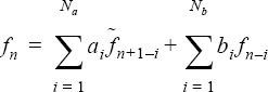
with the constraint that

MESH_MOTION( "dynamic rigid body with digital filter" ) {
   type                                = rigid_body_dynamic
   ...
   rigid_body_filter                   = iir
   rigid_body_iir_input_coefficients   = { 0.8, 0.8 }
   rigid_body_iir_output_coefficients  = { -0.6 }
}
The qualifiers of the SURFACE_OUPUT commands used to calculate the internal force and moment on the rigid body are listed in rigid_body_surface_outputs. Since for the CSS solution strategy the internal force and moment are updated only when the corresponding SURFACE_OUPUT command is evaluated, it is highly recommended that integrated_output_frequency be set to one in each of these commands for best accuracy. For the MIC strategy this frequency parameter is ignored; the internal forces and moments are updated as needed.
MESH_MOTION( "rigid platform" ) {
   type                                           = rigid_body_dynamic
   rigid_body_x_displacement                      = active
   rigid_body_y_displacement                      = active
   rigid_body_z_displacement                      = zero
   rigid_body_x_rotation                          = zero
   rigid_body_y_rotation                          = zero
   rigid_body_z_rotation                          = zero
   rigid_body_center                              = { 0, 0, 0 }
   rigid_body_direction                           = { 1, 0, 0 ;
                                                      0, 1, 0 ;
                                                      0, 0, 1 ; }
   rigid_body_mass                                = 1.2E+08
   rigid_body_stiffness                           = {6.4E+05,6.4E+05,0,0,0,0}
   rigid_body_damping                             = { 0, 0, 0, 0, 0, 0 }
   rigid_body_dyadic                              = { 0, 0, 0, 0, 0, 0 }
   rigid_body_rotational_stiffness                = { 0, 0, 0, 0, 0, 0 }
   rigid_body_rotational_damping                  = { 0, 0, 0, 0, 0, 0 }
   rigid_body_external_force                      = { 0, 3.E+07, 0 }
   rigid_body_external_force_multiplier_function  = none
   rigid_body_external_moment                     = { 0, 0, 0 }
   rigid_body_external_moment_multiplier_function = none
   rigid_body_initial_displacement                = { 0, 0, 0 }
   rigid_body_initial_velocity                    = { 0, 0, 0 }
   rigid_body_initial_rotation                    = { 0, 0, 0 }
   rigid_body_initial_angular_velocity            = { 0, 0, 0 }
   rigid_body_initial_force                       = { 0, 0, 0 }
   rigid_body_internal_force_multiplier_function  = none
   rigid_body_initial_moment                      = { 0, 0, 0 }
   rigid_body_internal_moment_multiplier_function = none
   rigid_body_filter                              = none
   rigid_body_surface_outputs                     = { "platform" }
}
NODAL_BOUNDARY_CONDITION( "all x-disp" ) {
   nodes                                          = Read( "all.nbc" )
   variable                                       = mesh_x_displacement
   type                                           = piecewise_linear
   curve_fit_variable                             = x_reference_coordinate
   curve_fit_values                               = { -175, 0. ;    # side1
                                                       -75, 1. ;    # side1 of platform
                                                       +75, 1. ;    # side2 of platform
                                                       +175, 0. ; } # side2
   mesh_motion                                    = "rigid platform"
 }
 NODAL_BOUNDARY_CONDITION( "all y-disp" ) {
   nodes                                          = Read( "all.nbc" )
   variable                                       = mesh_y_displacement
   type                                           = piecewise_linear
   curve_fit_variable                             = y_reference_coordinate
   curve_fit_values                               = { -175, 0. ;    # inflow
                                                       -75, 1. ;    # head of platform
                                                       +75, 1. ;    # tail of platform
                                                      +600, 0. ; }  # outflow
   mesh_motion                                    = "rigid platform"
}
EQUATION {
   mesh                                           = ale
   ...
}
   SURFACE_OUTPUT( "platform" ) {
   surfaces                                       = Read( "platform.srf" )
   shape                                          = four_node_quad
   element_set                                    = "sea"
   integrated_output_frequency                    = 1
}
The platform is allowed to move only horizontally and without any rotation. The equations and parameters corresponding to the other degrees of freedom are ignored. The wires preventing the platform from floating away are modeled by springs; the spring constants appear on the diagonal of the stiffness matrix. The atmosphere is not modeled directly but its effect on the platform is roughly modeled by an external force in the y direction. Since waves are modeled in the "sea" element set, commands not shown here, the z mesh displacement is nonzero. It is controlled by the free surface, other boundary conditions, and an ALE equation. The x and y components of the mesh displacement are controlled by the NODAL_BOUNDARY_CONDITION commands above. The effect of the curve fits is to smoothly vary the horizontal mesh displacements from zero at the outer boundaries to the MESH_MOTION values near the platform without having to solve an ALE equation for them.
In the above example, if the z mesh displacement could also be constrained, that is, there was no free surface, then there would be no mesh displacement degrees of freedom left to solve for in the ALE equation. In general, if all three components of the mesh displacement on all nodes are specified through the appropriate commands, then mesh=specified can be used in the EQUATION command and the solution of an ALE equation is eliminated (no stagger is needed for it). The appropriate commands are NODAL_BOUNDARY_CONDITION and SIMPLE_BOUNDARY_CONDITION, either with or without mesh_motion; and ELEMENT_SET using mesh_motion. In the latter case, all nodes in the element set are moved according to the specified MESH_MOTION command.
EQUATION {
...
    mesh                               = specified
...
}
ELEMENT_SET( "Fluid" ) {
…
    mesh_motion                        = "interpolated displacement"
…
}
MESH_MOTION( "interpolated displacement" ) {
    type                               = interpolated_motion
    interpolated_motion_surfaces       = {"top","bottom"}
}
INTERPOLATED_MOTION_SURFACE( "top" ) {
   surfaces                            = Read( "MESH.DIR/top.ebc" )
   shape                               = three_node_triangle
   element_set                         = "Fluid"
   type                                = faceted
}
INTERPOLATED_MOTION_SURFACE( "bottom" ) {
    surfaces                           = Read( "MESH.DIR/bottom.ebc" )
    shape                              = three_node_triangle
    element_set                        = "Fluid"
    type                               = faceted
}
For each node in the "Fluid" element set, AcuSolve computes the distance to the interpolated_motion_surfaces and scales its displacement based on the motions of the surfaces. This type of mesh motion is used in place of the ALE approach, or as a complement to it, to achieve mesh deformation in applications such as Fluid Structure Interaction. This is a rather simple method for deforming the mesh that has significant run time savings over using the ALE approach. Because of its simplicity, however, the method is limited in the extent of deformation that it can handle. More importantly, the motion of the mesh on every interpolated_motion_surfaces must be fully specified in all three directions. Consequently, free surfaces and guide surfaces cannot be used as interpolated motion surfaces.

In this example, nodes on the top or bottom surface are dominated by the interpolated mesh motion. If you want to constrain them within the planar surface where they are located initially, you have to put a slip-type simple boundary condition for mesh displacement or a zero nodal boundary condition for the component that is normal to the planar surface.
Another scenario is that both top and bottom surfaces are included in the driving surfaces as well. In that case you need to specify the motion of these two surfaces. If any component of the mesh displacement is missing, AcuSolve will just keep that component as its initial value. For example, you may set slip for the mesh displacement on the top surface, but you will not see any sliding motion of the nodes because interpolated mesh motion does nothing on nodes on interpolated_motion_surfaces or say driving surfaces. For the same reason, if you do not specify any mesh boundary condition for the top or bottom surface nodes there will just stay where they are initially throughout the simulation.
MESH_MOTION
    type                                = rigid_body_dynamic
    rigid_body_x_rotation               = active
    rigid_body_y_rotation               = zero
    rigid_body_z_rotation               = zero
    rigid_body_rotation_only            = on
    rigid_body_moment_arm               = {0, 0, -1.42}          #
local coordinates of center of mass
    rigid_body_external_force           = { 0.0, 0.0, -30*9.8; } #
gravity force in global coordinate system
    rigid_body_x_displacement           = zero
    rigid_body_y_displacement           = zero
    rigid_body_z_displacement           = zero
    rigid_body_center                   = { 2.0, 3.0, 4.0; }     #
rotation center