
FLEXIBLE_BODY
Specifies a solid body for fluid-structure interaction.
Type
AcuSolve Command
Syntax
FLEXIBLE_BODY("name") {parameters...}
Qualifier
User-given name.
Parameters
- equation (enumerated) [=mesh_displacement}
- Fluid-structure interaction modeling strategy.
- mesh_displacement or mesh
- Fluid mesh displacement boundary conditions.
- velocity or vel
- Fluid velocity boundary conditions.
- num_modes (integer) >0 [=1]
- Number of modes to model solid body dynamics.
- type (enumerated) [=trapezoidal]
- Flexible body type.
- trapezoidal
- Trapezoidal rule used for time integration.
- user_function or user
- Solid body deformation described by a user function.
- num_sub_steps (integer) >=1 (=1)
- Number of sub-steps in time integration. Used with trapezoidal type.
- mass (array) [={1}]
- Mass array of dimension num_modes. Used with trapezoidal type.
- stiffness (array) [={1}]
- Stiffness array of dimension num_modes. Used with trapezoidal type.
- stiffness_multiplier_function (string) [=none]
- User-given name of the multiplier function for scaling the stiffness. If none, no scaling is performed.
- damping (array) [={0}]
- Damping array of dimension num_modes. Used with trapezoidal type.
- damping_multiplier_function (string)[=none]
- User-given name of the multiplier function for scaling the damping. If none, no scaling is performed.
- contact_constraints (array) [={}]
- Array of constraints that limit the motion of the solid body. Used with trapezoidal type.
- external_force (array) [={0}]
- External force array of dimension num_modes.
- external_force_multiplier_function (string) [=none]
- User-given name of the multiplier function for scaling the external force. If none, no scaling is performed.
- initial_displacement (array) [={0}]
- Initial displacement array of dimension num_modes.
- initial_velocity (array) [={0}]
- Initial velocity array of dimension num_modes.
- initial_force (array) [={0}]
- Initial force array of dimension num_modes.
- internal_force_multiplier_function (string)[=none]
- User-given name of the multiplier function for scaling the internal force. If none, no scaling is performed.
- user_function or user (string) [no default]
- Name of the user-defined function. Used with user_function type.
- user_values (array)[={0}]
- Array of values to be passed to the user-defined function. Used with user_function type.
- surface_outputs (list) [={0}]
- Array of SURFACE_OUTPUT command qualifiers used to calculate the force and moment on the solid body.
- evaluation (enumerated) [=once_per_time_step]
- Frequency of evaluating the external forces.
- once_per_solution_update or often
- Every solution update.
- once_per_time_step or step
- Every time step.
- filter (enumerated) [=none]
- Type of filter to smooth the external forces.
- none
- No filter.
- iir
- Infinite impulse response digital filter. Requires iir_input_coefficients and iir_output_coefficients.
- iir_input_coefficients (array) [={1}]
- Infinite impulse response digital filter coefficients applied to computed values. Used with iir filter.
- iir_output_coefficients (array) [={}]
- Infinite impulse response digital filter coefficients applied to previously filtered values. Used with iir filter.
Description
- Flow induced vibration of a solid wall and coupling to computational aero-acoustics (CAA).
- VIV (vortex induced vibration) modeling of oil platform risers.
- Deformation of vein walls due to pulsing blood flow.
FSI is defined as simulating the bidirectional interaction (coupling) between a fluid flow and a deforming solid/structural model. This definition is very specific. It does not include other types of couplings such as fluid with thermal solid/structures or fluid with rigid body dynamics, both of which are already available through other commands in AcuSolve. The coupling may be very complex depending on the degree of deformation of the solid/structure, especially for large deformations leading to nonlinear solid/structure stress/strain behavior. Here, only linear solid/structural deformation is considered that can be represented by the linear finite element dynamic systems of equations:
where , v, and d are the nodal acceleration, velocity, and displacement fields respectively; M, C, and K are the matrices of mass, damping, and stiffness; and F is the external force. The linearity assumption means the matrices M, C, K, and F are independent of the solution d (and its first and second time derivatives, v and ). Given this assumption, the above equation of motion may be decomposed into its eigen modes:
where is the ith eigenvalue of the above system with eigenvector Si . The number of modes in the finite element model of the solid/structure is given by num_modes. Projection of the equation of motion into the eigenspace yields:
where y is the vector of amplitudes, henceforth referred to as the "displacements" of the eigen modes, a dot represents the time derivative, and
The damping matrix C is assumed to be in the above eigen space. This is actually a minor assumption, since for most problems C is either zero or proportional to K. This also means that the matrix c is diagonal. If this is not quite right, only the diagonal part of c is used.
The above equation for y is a set of num_modes independent ordinary differential equations (ODEs). To solve it, F needs to be computed first and projected to f. Each component of y and its time derivatives can then be solved for. From the solution, the original dependent variables can be reconstructed:
A further simplifying assumption is made that only a limited number of eigen modes is needed from the above system to produce a good representation of the solid deformation to be coupled with the fluid flow.
- Solid model: A solid/structural finite element model must first be created. The first num_modes eigen modes of this model is computed. This step is performed with an existing linear solid/structural code, such as OptiStruct, Abaqus, ANSYS, Nastran, or other means. Analytic solutions may of course be used if available. This gives a set of eigenvalues and eigenvectors on the solid mesh.
- Projection: Next, an independent fluid mesh is created, and the fluid surfaces that are in contact with the solid are identified. The eigenvectors from the surfaces nodes of the solid mesh are then projected to the surface nodes of the fluid mesh. The AcuPev program is a tool to facilitate this process; see the AcuSolve Programs Reference Manual for details. An analytic solution may be possible for simple problems.
- AcuSolve: The projected eigen system is entered into AcuSolve, which will then solve the transient coupled linearized deformation and the fluid flow. The process is somewhat similar to the current AcuSolve solution of coupled rigid body dynamics (see MESH_MOTION with type=rigid_body_dynamic).
FLEXIBLE_BODY( "riser" ) {
   equation                                 = mesh_displacement
   num_modes                                = 5
   type                                     = trapezoidal
   mass                                     = { 1, 1, 1, 1, 1 }
   damping                                  = { 0, 0, 0, 0, 0 }
   damping_multiplier_function              = none
   stiffness                                = { 1, 1.5, 3.2, 6.8, 12.6 }
   stiffness_multiplier_function            = none
   external_force                           = { 0, 0, 0, 0, 0 }
   external_force_multiplier_function       = none
   initial_displacement                     = { 0, 0, 0, 0, 0 }
   initial_velocity                         = { 0, 0, 0, 0, 0 }
   initial_force                            = { 0, 0, 0, 0, 0 }
   internal_force_multiplier_function       = none
   surface_outputs                          = { "side wall", "bottom wall" }
   evaluation                               = once_per_time_step
   filter                                   = none
}
The type of modeling is given by equation which may be either mesh_displacement or velocity; see below. The number of eigen modes is given by num_modes, which is also the dimension of all arrays in this command. The time integration strategy is given by type; time integration is performed internally for type=trapezoidal. See below for type=user_function. The diagonal of the mass matrix m is given by mass, which is typically a vector of ones. The diagonal of the stiffness matrix k is given by stiffness, which is typically the vector of eigenvalues. The diagonal of the damping matrix c is given by damping; c in turn is given by the projection of C onto the eigenvectors matrix. Forces not induced by the fluid, such as back pressure, may be given by external_force, which may be scaled with external_force_multiplier_function. The initial conditions are given by initial_displacement and initial_velocity. The initial fluid force is given by initial_force. These last three parameters will be reset at restart. The surfaces used to compute the fluid forces, that is, F, applied to the solid are given by surface_outputs, which references one or more SURFACE_OUTPUT commands. The fluid forces may be scaled with internal_force_multiplier_function. The usual use for this is to ease into a fluid/structure simulation by implementing a multiplier function that starts at zero and ramps up to one.
NODAL_BOUNDARY_CONDITION( "mesh_x_displacement on side wall" ) {
   nodes                               = Read( "riser.side-wall.nbc" )
   variable                            = mesh_x_displacement
   type                                = flexible_body
   flexible_body                       = "riser"
   nodal_modes                         = Read( "riser.side-wall.xeig" )
}
The first parameter is the usual list of nodes. variable may be any of the four mesh displacement variables or any of the four velocity variables, depending on the type of modeling; see below. The direction variables also require the usual direction parameters, including direction_type. A flexible_body type indicates that this boundary condition is used as part of a FSI coupling. The corresponding FLEXIBLE_BODY command is provided by flexible_body, which in particular provides num_modes. The eigenvectors Si are given by nodal_modes, which contains num_modes+1 columns corresponding to the node number and the num_modes eigenvectors. The set of nodes in nodal_modes must be the same as in nodes. The eigenvectors are used for two purposes: to project F to form the modal force f; and to form d and v, which are needed for fluid boundary conditions.
- Conventional Sequential Staggered (CSS): This uses a single-pass of displacements and forces at each time step. The result is essentially an explicit scheme since the data comes from the previous time step. CSS is used when there is exactly one nonlinear stagger per time step (max_stagger_iterations=1 in the STAGGER command).
- Multi-Iterative Coupling (MIC): This strategy corrects the interfacial forces via a multi-pass transfer of mesh displacements and fluid forces. From numerical experiments, robustness and efficiency of the scheme is obtained for a mass-density ratio of O(1). The scheme requires at least two nonlinear stagger iterations per time step. The interfacial force and displacement residuals can be obtained by printing the *.Log file (generated by AcuRun) with a verbose level of two.
The parameter contact_constraints may be used to specify a set of contact conditions to be imposed on the time evolution of the flexible body. Only simple contact between a set of points attached to the flexible body with a set of fixed rigid planes is accommodated. Contact constraints are supported only with trapezoidal type. Contact introduces a strong nonlinearity on the linear model given above, and thus must be modeled with care.

The contact condition may then be written as
where d0 = d0(t) is the displacement of the flexible body as a function of time at point x0. Recall that the displacement is the sum of contributions from each mode of the flexible body; in other words:

where yi is the displacement of the i-th mode, and Si is the i-th eigenvector of the flexible body at point x0 . Combining the above two equations yields:

which may be simplified to:


Formally, the solution for the displacement of the flexible body with contact is the transient solution for y subject to the inequality constraints above. This system may be solved using the "interior point method" of "quadratic programming".
In addition to the above constraint on the modal displacement field, the "restitution coefficient", denoted by , is used to impose the following condition on the modal velocity field when the contact condition occurs:

where  and
and  are the modal
velocities at time step n and n+1, respectively, and the contraction is over all of the
modes. The above equation approximately sets the
c component of modal velocity after contact
occurs to the negative of the corresponding modal velocity prior to contact scaled by
the restitution coefficient.
are the modal
velocities at time step n and n+1, respectively, and the contraction is over all of the
modes. The above equation approximately sets the
c component of modal velocity after contact
occurs to the negative of the corresponding modal velocity prior to contact scaled by
the restitution coefficient.
The parameter contact_constraints is a two dimensional array with num_modes+2 columns, corresponding to the vector c (num_modes columns), the b value, and the restitution coefficient, . Each row of the array corresponds to one contact constraint. This array is usually constructed using the contact_constraints_file option of AcuPev; see the AcuSolve Programs Reference Manual.
FLEXIBLE_BODY( "body with simple contact" ) {
   equation                            = mesh_displacement
   num_modes                           = 2
   ...
   num_sub_steps                       = 4
   contact_constraints                 = { +0.2, +0.1, -0.1, 0.6 ;
                                           -0.2, -0.1, -0.15, 0.6 ; }
}
The b values for both conditions above are negative. This is expected. In general, if a flexible body at its reference condition, that is, with no deformation, is not in contact, then all b values will be negative. If the flexible body is in contact at its reference position, then the b value(s) corresponding to the contact point(s) will be zero.
You must be very careful in modeling a FSI problem with the above contact_constraints parameter. There are three main sources of error.
By far the most important source of error is the validity of the flexible body shape as modeled by a limited number of modes when contact occurs. You can typically use fairly small number of modes to accurately model the interaction between a fluid and a flexible body under normal conditions. But contact may require a different set of modes in order to accurately model the shape of the flexible body. When contact occurs, the rigid plane effectively imposes a force on the flexible body. This force is imposed at the point of contact (point x0 above). The shape of the flexible body under the influence of contact is as valid as to the degree in which the contact force is represented by the eigenvectors. Let the contact force be given by Fi=Fi(x) . The error in the representation of this force is given by:

The second source of error is in modeling of the disruptive effect of contact on the fluid forces. In other words, when contact occurs, the flexible body rapidly stops or even reverses direction. This typically causes a rapid change in fluid forces. To minimize the inaccuracy caused by this effect, smaller time increments in the fluid solution may be required.
The final source of error is in the time evolution of the flexible body itself, that is, the contact may occur in the middle of a time step. Thus the flexible body motion within the time step is approximated as is the fluid motion. A partial correction to the body motion but not the fluid motion can be added. The parameter num_sub_steps is introduced for this, which is only available for trapezoidal type. The flexible body time evolution is solved with num_sub_steps substeps within each fluid time step. Higher values of this parameter provides more accurate modeling of the discontinuities introduced by contact.
FLEXIBLE_BODY( "baffle" ) {
   equation                            = mesh_displacement
   num_modes                           = 1
   type                                = user_function
   surface_outputs                     = { "baffle" }
   user_function                       = "usrClientServer"
   user_strings                        = { "usrFSI.pl" }
}
where the user function is implemented in the perl script usrFSI.pl which is controlled through the client/server mechanism. See the AcuSolve User-Defined Functions Manual.
#include "acusim.h"
#include "udf.h"
UDF_PROTOTYPE(usrClientServer) ;
Void usrClientServer(        UdfHd     udfHd,
                             Real*
                                       outVec,
                             Integer   nItems,
                             Integer   vecDim )

{

char          buffer[1024] ;           /* a string buffer                          */
char*         name ;                   /* name of the UDF                          */
Integer       i ;                      /* a running index                          */
Real*         disp ;                   /* displacement (curr or prev)              */
Real*         dispC ;                  /* next displacement                        */
Real*         extForce ;               /* external force                           */
Real*         intForce ;               /* internal force                           */
Real*         timeInc ;                /* time increment                           */
Real*         usrVals ;                /* user supplied values                     */
Real*         vel ;                    /* velocity (curr or prev)                  */
Real*         velC ;                   /* next velocity                            */
String        command ;                /* execution command                        */
String*       usrStrs ;                /* user supplied strings                    */
udfCheckNumUsrVals(                    udfHd,                      0              ) ;
udfCheckNumUsrStrs(                    udfHd,                      1              ) ;
usrVals       = udfGetUsrVals(         udfHd                                      ) ;
usrStrs       = udfGetUsrStrs(         udfHd                                      ) ;
command       = usrStrs[0] ;
name          = udfGetName(            udfHd                                      ) ;
timeInc       = udfGetTimeInc(         udfHd                                      ) ;
dispC         = outVec ;
velC          = outVec + nItems ;

/* Start the client */
   if ( udfFirstCall(udfHd) ) {
   udfOpenPipePrim(                    udfHd,                        command      ) ;
   }

/* If the first time step */
   if ( udfFirstStep(udfHd) ) {
   disp       = udfGetFbdData( udfHd, name, UDF_FBD_CURR_DISPLACEMENT             ) ;
   vel        = udfGetFbdData( udfHd, name, UDF_FBD_CURR_VELOCITY                 ) ;
   for ( i = 0 ; i < nItems ; i++ ) {
       dispC[i]    = disp[i] ;
       velC[i]     = vel[i] ;
   }
       return ;
}

/* Otherwise, get the data from the external program */
   intForce    = udfGetFbdData( udfHd, name, UDF_FBD_INTERNAL_FORCE               ) ;
   extForce    = udfGetFbdData( udfHd, name, UDF_FBD_EXTERNAL_FORCE               ) ;
   disp        = udfGetFbdData( udfHd, name, UDF_FBD_PREV_DISPLACEMENT            ) ;
   vel         = udfGetFbdData( udfHd, name, UDF_FBD_PREV_VELOCITY                ) ;
   for ( i = 0 ; i < nItems ; i++ ) {
       udfWritePipe(   udfHd,        "%d %.16g %.16g %.16g %.16g %.16g            ",
                       i,            timeInc,        disp[i],
                       vel[i],       intForce[i],    extForce[i]                  ) ;
}
for ( i = 0 ; i < nItems ; i++ ) {
       udfReadPipe(    udfHd,        buffer,         1024                         ) ;
       sscanf(         buffer,       "%le %le",      &dispC[i],
                       &velC[i]                                                   ) ;
}

} /* end of usrClientServer() */#!/usr/bin/env perl
$| = 1 ;
if ( scalar(@ARGV) != 0 ) {
die "Usage: $0" ;
}
# Hard code matrices
@mass = ( 200. );
@damp = ( 0. );
@stiff = ( 50. );
$doLog = 0 ;
if ( $doLog ) {
open( LG, ">fsi.log" ) || die "unable to open fsi.log" ;
}
# Loop through the steps/modes and advance
while( <> ) {
chomp ;
( $indx, $timeInc, $dispP, $velP, $intF, $extF ) = split( /\s/, $_, 6 ) ;
print LG "< $indx $timeInc $dispP $velP $intF $extF\n" if $doLog ;
$timeInc != 0 || die "timeInc == 0" ;
$fct1 = $mass[$indx] / $timeInc ;
$fct2 = $damp[$indx] * 0.5 ;
$fct3 = $stiff[$indx] * $timeInc /4. ;
$fct4 = $stiff[$indx] ;
$rhs = $intF + $extF
+ $fct1 * $velP
- $fct2 * $velP
- $fct3 * $velP
- $fct4 * $dispP ;
$lhs = $fct1 + $fct2 +$fct3 ;
$lhs != 0 || die "lhs == 0" ;
$velC = $rhs / $lhs ;
$dispC = $dispP + $timeInc * ( $velP + $velC ) / 2 ;
printf "%.16g %.16g\n", $dispC, $velC ;
print LG "> $dispC $velC\n" if $doLog ;
}Note the use of the function udfGetFbdData(). This is similar to udfGetOsiData(), except it provides the solution data for a given FLEXIBLE_BODY command. See the AcuSolve User-Defined Functions Manual for a list of valid data names. outVec is used to return both the displacement and velocity at step n+1.
The evaluation parameter controls how often the external force vector on the solid body is updated. Setting this to once_per_time_step freezes the external force for the rest of the time step.
once_per_solution_update updates the external force every time the fluid solution is updated.
The computed projected forces of AcuSolve may be smoothed in time by applying a digital filter before using the forces for computing the modal response. An iir filter gives an infinite impulse response filter, which is defined by:
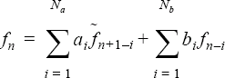
with the constraint that:

FLEXIBLE_BODY( "FSI with digital filter" ) {
   ...
   filter                    = iir
   iir_input_coefficients    = { 0.8, 0.8 }
   iir_output_coefficients   = { -0.6 }
}- equation=mesh_displacement. ALE or specified mesh must be used. The NODAL_BOUNDARY_CONDITION commands containing type=flexible_body must impose boundary conditions on components of the mesh displacement. The fluid velocity is then matched to the mesh motion via other NODAL_BOUNDARY_CONDITION commands.
- equation=velocity. Modeling of the mesh deformation is assumed to be not important and thus its effect may be approximated through velocity boundary conditions on the wall. The NODAL_BOUNDARY_CONDITION commands containing type=flexible_body must impose boundary conditions on components of the velocity.
- The displacement or velocity values of the eigen modes are used to compute new boundary condition values for the mesh displacement or fluid velocity variables at each node of the flexible body NODAL_BOUNDARY_CONDITION commands.
- At the end of each time step, the forces on the surfaces listed in surface_outputs are computed. The nodal values of the forces are multiplied by the eigenvectors to compute the internal forces on the flexible body. In other words, the force field applied by the fluid is projected into the eigen space of each mode. This force is added to the external force and the result is used to advance the displacement or velocity of each mode.
The MIC strategy consists of the same two steps executed every nonlinear stagger iteration with the forces and displacements also updated every stagger instead of every time step.
- All three components of mesh displacement (or velocity) may be specified, or just two components, or even just the normal component.
- Mathematically, however, if a direction boundary condition is used, either only one boundary condition per node should be used, or care must be taken to ensure orthogonal components. Otherwise, error in the accumulation of the contribution to the force f may occur.
- You must be careful when using direction boundary condition with mesh displacement, since the eigenvectors may only be valid for a particular direction, and the mesh may shift as a result of the boundary condition.
- The collection of nodes in the NODAL_BOUNDARY_CONDITION commands corresponding to a particular FLEXIBLE_BODY command may be a subset or a superset of the nodes contained in the surface_outputs list. If a boundary condition node does not have a corresponding surface output node, then that node does not contribute to f, but the flexible body does control its motion. This may be used, for example, to define the motion of all nodes in the problem, while only a subset contribute to the solid deformation. A less useful scenario is a node in the surface_outputs list not appearing in any nodal boundary condition. Probably the only valid case is when this node has other boundary conditions that take precedence. In either case, a warning message will be issued.
- Currently, a zero intersection between these two sets of nodes, flexible body nodal boundary conditions and the surface output list, is disallowed, even though a case can be envisioned where a flexible body independent of any fluid force is used just as a simple mechanism to move the nodes.
- The precedence parameter in a NODAL_BOUNDARY_CONDITION command may be used to suppress a FSI boundary condition on a node.