Constraints

Introduction

In the data tree of Flux the node Solver > Optimization > Constraints allows the user to define some constraints which are structural or physical limitations imposed by the optimizer, a constraint allow the user to control the shape of the design with some symmetries constraints, volume values constraints or physical limits. The short list of the constraints is given below:
Table 1. Table summarizing all the constraints available in Flux
Constraints Required information
Physical constraint
  • Select a Predefined function
  • Or a Compose function which requires:
    • A Compose type file
    • The name of the function related to the constraint
  • Select the input responses which are described as physical depending responses
  • Lower or an upper bound in the same unit as the response (both are not mandatory)
Constraints on 2D faces volume
  • A common percentage factor of variation


    Figure 1. Vmax and Vmin are the upper and lower bounds, p_var the common factor
  • A percentage factor for the lower bound and another factor for the upper bound


    Figure 2. Vmax and Vmin are the upper and lower bounds, p_max and p_min the factors for the upper and lower bounds
  • The values for lower and upper bounds


    Figure 3. Vmax and Vmin are the upper and lower bounds, p_max and p_min the values for the upper and lower bounds
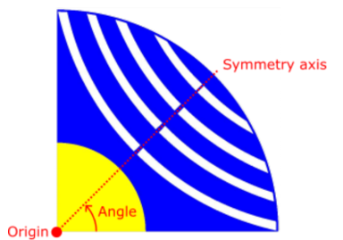
Symmetry constraint (defined by direction)
  • The origin of the symmetry axis,
  • The direction of the axis.


Figure 4. Origin point and a simple symmetry axis over the rotor of a rotating machine
In this case, the direction of the symmetry axis is (0.5;0.5).
Symmetry constraint (defined by angle)
  • The origin of the symmetry axis,
  • The angle of the axis.


Figure 5. Origin point and a simple symmetry axis over the rotor of a rotating machine
In this case, the angle of the symmetry axis is 45°.
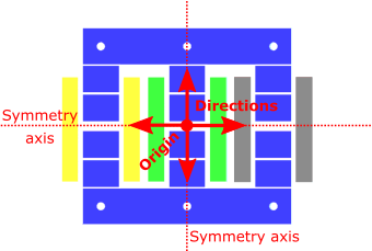
Double symmetry constraint (defined by direction)
  • The origin of the symmetry axis,
  • The direction of one of the axes, the second axis is automatically taken perpendicular to the first one.


Figure 6. Origin point and double symmetry axis over an electromagnetic device
In this case, only one of both axes must be defined, choose between (1;0) for X axis or (0;1) for Y axis.
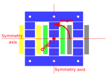
Double symmetry constraint (defined by angle)
  • The origin of the symmetry axis,
  • The angle of one of the axes, the second axis is automatically taken perpendicular to the first one.


Figure 7. Origin point and double symmetry axis over an electromagnetic device
In this case, only one of both angles must be defined, one can choose between 0, 90, 180, 270, ….