Solving options and methods for estimating the current density in 3D coil conductor regions

Introduction

Flux must evaluate the current density J in coil conductor regions at certain points during the solving process and while the user is post-processing the solution. Evaluating this quantity may be particularly challenging in 3D projects containing this kind of region due to the geometrical complexity of the coils in the device (or, more specifically, of the volumes assigned to the coil conductor regions).

Since a unique and exact FEM-based approach for computing the current density in complex-shaped conductors is not available, approximate but accurate techniques become necessary.

Since the choice of the best technique depends on several aspects, Flux provides the user with an automatic solving option to get results in a faster, easier way. On the other hand, an experienced user is also allowed to explicitly choose between two current density evaluation methods, which are available among the solving options of a Flux project.

These solving options and methods are discussed in this chapter, which covers the following topics:

adjustments of the solving options;
discussion on the geometry constraints that the volumes assigned to a coil conductor region must satisfy;
outline of the current density computation methods used by Flux 3D.

Adjusting the solving options for current density evaluation

Flux 3D is able to automatically choose among two current density evaluation methods. However, the technique to compute the current density in coil conductor regions may be modified if desired by changing a solving option called Method for the computation of J in coil conductor regions in 3D prior to the resolution.

To navigate to this list of options in Flux 3D, the user must open the Solving menu and perform the following choices: Solving process options > Edit > Advanced tab. The user may then choose one of the three approaches from that list:

Automatically specified method: the default method, which is preselected when the project is created. Depending on the geometry of the coil conductor regions in the project and on their physical subtypes (i.e., coil conductor regions without losses, with losses and simplified geometrical description and with losses and detailed geometrical description), Flux 3D will automatically choose between the two available methods that are described in the following points 2 and 3. Further details on the automatic choice are provided at the end of this section.
Analytical method or by interpolation from lines: a method that is applicable to all subtypes of coil conductor regions in Flux 3D. However, Flux 3D may only employ this method if the volumes assigned to the coil conductor regions satisfy significant geometrical constraints.
Method with electric conduction resolution (with finite element method) + uniform J norm: this method admits coil conductor regions assigned to volumes that are subjected to fewer geometrical constraints. However, Flux 3D may only apply it to coil conductor regions without losses and to coil conductor regions with losses and simplified geometrical description.

The behavior of the first (default) solving option Automatically specified method is as follows:

In the cases of a Coil conductor region without losses or of a Coil conductor region with losses and simplified geometrical description.
- If the geometry of the coil conductor region is compatible with the Analytical method or by interpolation from lines, then Flux 3D applies it in the evaluation of the current density.
- Otherwise, the Method with electric conduction resolution + uniform J norm is used.
For a Coil conductor region with losses and detailed geometrical description, the Analytical method or by interpolation from lines is used.

This behavior is also summarized in the following table:


Type of volume region	Geometry compatible with the "Analytical method or by interpolation from lines"	Method used for the computation of J
Coil conductor region without losses or Coil conductor region with losses and simplified geometrical description.	Yes	Analytical method or by interpolation from lines
	No	Method with electric conduction resolution (with finite element method) + uniform J norm
Coil conductor region with losses and detailed geometrical description.	Yes	Analytical method or by interpolation from lines
	No	Flux displays an error message during resolution.

Geometrical constraints and the applicability of each method

The available methods used by Flux 3D to compute the current density are only applicable if a certain number of geometrical constraints are satisfied, accordingly with the previous section.

The most significant constraint that rules their applicability is related to the shape of the volumes assigned to a coil conductor region. More specifically, their cross sections (i.e., the sections orthogonal to the current flow):

must not change their shapes between the input and output terminals for the Analytical method or by interpolation from lines to apply.
are allowed to vary between certain limits between the input and output terminal for the Method with electric conduction resolution (with finite element method) + uniform J norm to apply.

Other geometrical constraints affecting their applicability are related to:

the origin of the geometrical entities, that is, if the coil conductor region is assigned to volumes whose geometrical entities were imported into the Flux project from a CAD file or created in Flux's own modeler;
the structured character of the geometric objects, that is, if the coil conductor region contains "parasite" or "unstructured" points, lines and faces anywhere in its volumes (i.e., as if they were not generated by an extrusion);
if the volumes in the coil conductor region share a common interface with other parts of the simulated device (e.g., the magnetic circuit of the coil);
the coil conductor region has input and output terminals with different numbers of faces.

In case any of these constraints is not respected, Flux 3D prompts the user with suitable warnings.

Outline of the solving methods for current density evaluation

The following subsections outline the two solving methods for evaluating the current density in coil conductor regions in Flux 3D that were previously introduced in this chapter.

Analytical method or by interpolation from lines

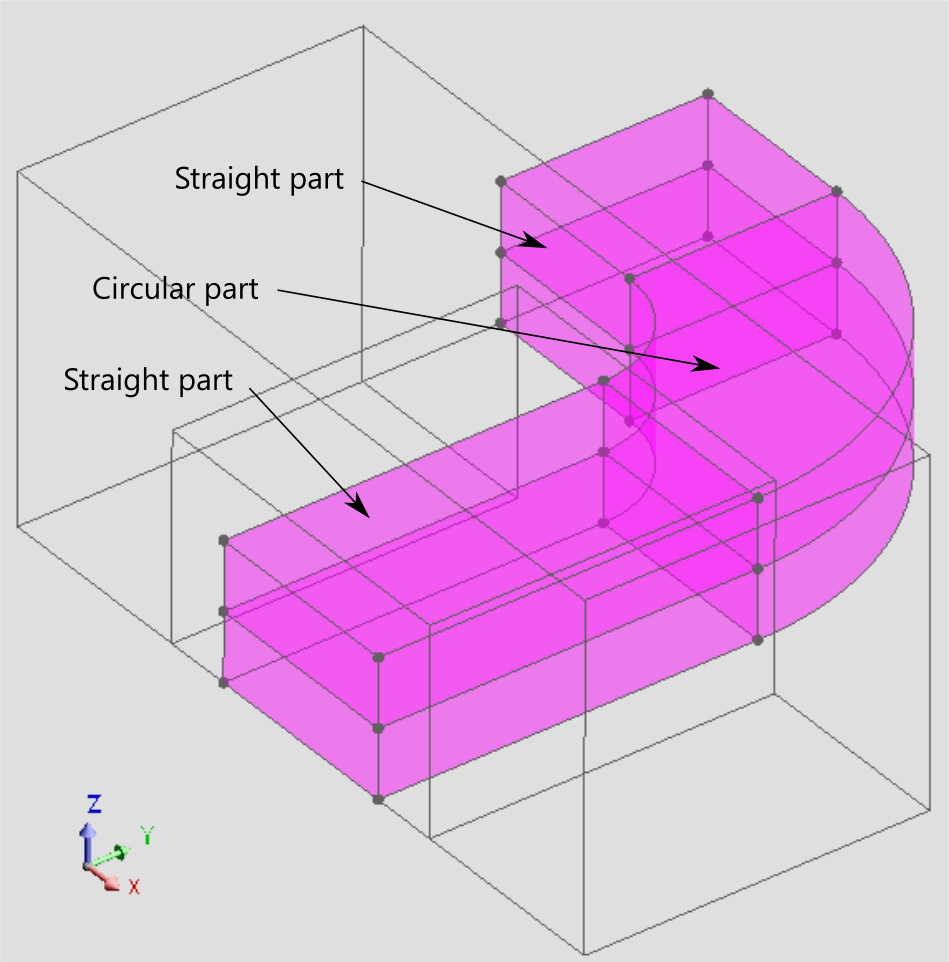
In this approach, the geometry of the coil conductor region must have a constant cross-section, as if the faces of the input electric terminal had been extruded along the current path towards the output terminal (as depicted in Figure 1).

Under such circumstances, the current density is computed with simple analytical formulas or by an interpolation method, depending on the nature of the geometrical entities (i.e., if they were created by the user through Flux internal modeler or if they were imported from a CAD file).

Figure 1. Coil geometry with straight and circular parts exhibiting a constant cross-section.

Method with electric conduction resolution (with finite element method) + uniform J norm

At the beginning of the solving process, a finite element computation of an electric conduction problem is performed in each coil conductor region. The electric scalar potential V is used as state variable and a resistivity of 1 Ω.m is admitted. The values of V at each node are stored.

During the solving process or while in post-processing, the current density J is computed at a point from V, with formula J = -grad V. Then the direction of J is kept, but its norm is adjusted. The latter results uniform in the whole region, with a value that depends on the section areas of the electric terminals, the number of turns of the coil, the number of wires in parallel and the coefficient for coils flux computation related to the existence of symmetries or periodicities.

This method also performs a test at the beginning of the solving process to verify if the coil conductor regions have constant or varying cross sections (as shown in Figure 2). Flux 3D solves a preliminary electric conduction problem for each coil conductor region in the project, supposing an imposed current of 1 A and a homogeneous and isotropic resistivity of 1 Ω.m. These computations yield the current density J_1A and the scalar electric potential V in each coil conductor region.

Figure 2. Coil geometry exhibiting a varying cross-section. The current density in the associated coil conductor region in Flux 3D may be evaluated with solving option "Method with electric conduction resolution (with finite element method) + uniform J norm".

Then the Joule losses P₁ and P₂ in each coil conductor region are computed in two different ways, with the same current of 1 A flowing in the coils:

P₁ = ꭍ_Ω |J_1A|² dΩ, in which J_1A is the current density in the coil and Ω represents the volume region,
P₂ = ꭍ_Ω |J_u|² dΩ, in which J_u is a current density in the coil with a uniform norm given by J_u = (N/S)*J_1A /|J_1A |. In this last expression, N is the number of turns in the coil and S is the arithmetic mean between the areas of the cross-sections orthogonal to the current density of the input and output terminals.

Flux 3D computes the deviation between P₁ and P₂ from these values with the formula below:

deviation = |P₁-P₂|/[2*(P₁+P₂)]

If the deviation yielded by this formula for a given coil conductor region results higher than 4%, then its cross-section is considered non constant between the input and output terminals. The software will then display the following warning:

Warning: Volume region: COIL_A. The area of the section orthogonal to the current density seems not constant when going from the input terminal to the output terminal. Please carefully verify your results. The current density may be wrong (see the user guide).