EDEM Analyst - Analyze Your Results
Learn how to review, examine, and analyze the results of the simulation using EDEM Analyst.
-
Click the
 icon
on the Toolbar.
icon
on the Toolbar.
-
Use the controls
 below the simulation window to rewind the simulation to the first Time
Step.
below the simulation window to rewind the simulation to the first Time
Step.
-
Click the
 icon to play through each Time Step of your simulation.
Configure the Display
You can use the Display section in the Analyst Tree to configure the appearance of the different elements in your model. The Geometry, particles, and contacts within your model can also be colored in a variety of ways. Any section of a Geometry, particle, contact type, or selection group can be colored independently.
-
Configure the Geometries subsection.
- Click Display in the Analyst Tree and then expand the Geometries subsection.
- Change the Geometry display by modifying the Display Mode options in the Geometry section.
- Select the Display Mode as Filled, Mesh, or Points.
- Specify the Opacity with values between 0-1, with 0 being completely transparent and 1 being solid.
- Click Apply All to view the changes in the Viewer window.
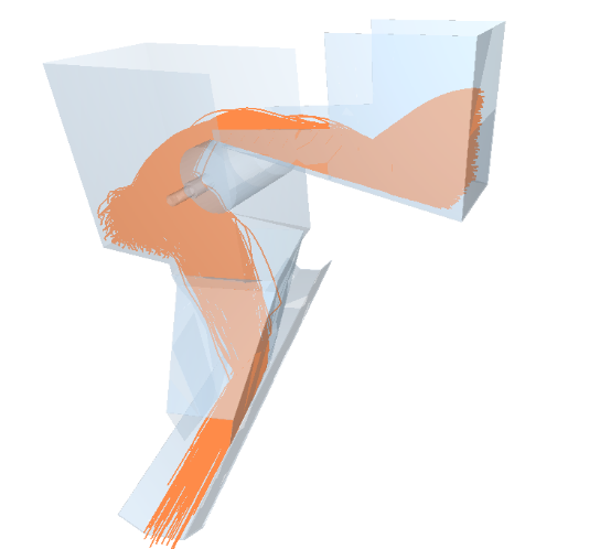
- Select the Display Mode as Filled with Opacity of 0.3 to view the flow of particles.
- Click Apply All.
- Before finishing, click factory_plate in the Geometries section and ensure that the Display factory checkbox is not selected.
- Click Apply if the Auto Update checkbox is not selected, else the changes will be applied automatically.
-
Configure the Particles subsection.
You can modify the display of the particles in a similar way as that of the Geometry. In addition, the particles can be represented using a number of different forms, such as cones, streams, and vector that traces the direction in which the particles move.
- Select the Particles subsection in the Analyst Tree.
- Select Vector from the Representation type dropdown list.
- Click Apply All.
- Change the Time Steps to review the flow of the material.
- Select Stream from the Representation type dropdown list.
- Click Options.
- In the Streams section, towards the bottom,
select the Stream All Steps and Stream
Fade checkboxes.
- Click the
 icon to rewind the simulation.
 - Click the icon to view how the direction of movement
of the particle changes over time.
- Click the
 icon at any point and set the
Representation type back to
Default.
icon at any point and set the
Representation type back to
Default.
Color Elements
You can color particles, Geometry and contacts within your model in a variety of ways. Any section of Geometry, particle, contact type, or selection group can be colored independently.
-
Color the Geometry according to the section type.
- Select the Feed_Conveyor Geometry element in the Analyst Tree.
- In the Coloring section of the Detailed View, select Velocity from the Color by dropdown list.
- Set the Min, Mid, and Max colors to the Blue, Green, and Red respectively.
- For Min Value and Max Value, select the Auto Update checkboxes.
- Repeat the same steps for Receiving_Conveyor and Head_Pulley Geometry elements.
- Click the icon to rewind the simulation, if
required.
- Click the icon to view the velocity of moving parts
of the Geometry.
- Before continuing, select the Geometries in the Analyst Tree.
- In the Coloring section, select Uniform from the Color bydropdown list.
- Select Color to Default from the Color dropdown list and then click Apply All.
-
Color the particles according to their velocity.
- Select Particles in the Particles subsection of the Analyst Tree.
- In the Coloring section of the Detailed View, select Velocity in the Color by dropdown list.
- Click next to the Min Value and Max Value fields to read the current values from the point in the simulation displayed in the Viewer.
- Select the Auto Update checkbox so that the values continue to update while the simulation is being played.
- Click Apply All to color the particles.
- Select the rock particle in the Analyst Tree.
- Select the Show Legend checkbox.
- Click Apply.
- Rewind the simulation back to the start and click the icon to view how the colors are updated as
the simulation progresses.
Create Selections
Selections allow data to be extracted from a particular area or element in the domain. Using selections, you can monitor any element passing through a particular area (known as a 'bin') or track particular elements wherever they move within the domain. You can then display, color, graph or export data based on the selections.
-
Create a mass flow sensor.
You can examine the mass flow over time in the bottom conveyor by including a mass flow sensor.
- Right-click Setup Selections in the Analyst Tree.
- Select .
- In the Representation section, set the Display Mode to Always.
- Set the properties of the bin group as follows:
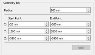
- Click Apply.
-
Create a grid bin group.
You can also examine the increase of mass over time on the rock box. To do so, you will need to create a bin group over it.
- Right-click Setup Selections in the Analyst Tree.
- Navigate to and name it .
- Select the newly created grid bin group and in the Detailed View, set
its properties as follows:
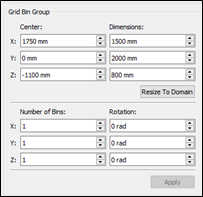
- Click Apply
-
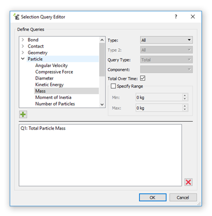
Define the Selection group queries.
A query is used to define a single element attribute, for example particle velocity, total force on a Geometry section, or number of collisions.
- To determine the total mass of particles accumulating in the rock box, use the controls at the lower section of the Viewer window or type the current time to 0s (the beginning of the simulation, when no particles are present in the rock box).
- Select Rock_Box_group in the Setup Selections section of the Analyst Tree.
- In the Options section of the Detailed View,
click Edit….
The Selection Query Editor is displayed.
- Expand Particle and then select Mass.
- Select All from the Type
dropdown list.
You can also select one of the particles from the Type dropdown list to monitor only that particle type.
- Set the Query Type to Total.
- Select the Total Over Time checkbox and click the
 icon.
icon. - Click OK. The query is displayed in the dialog box.
Note: You will not need to create a query for the mass flow sensor. -
Set the Selection group display options.
- In the Setup Selections section of the Analyst Tree, select Rock_Box_group.
- In the Representation section of the Detailed
View, click Edit... to edit the display
options.
The Display Options dialog box is displayed.
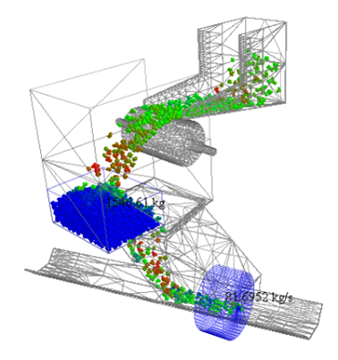
- Select the On-Screen Query checkbox to display
the mass in the Viewer:
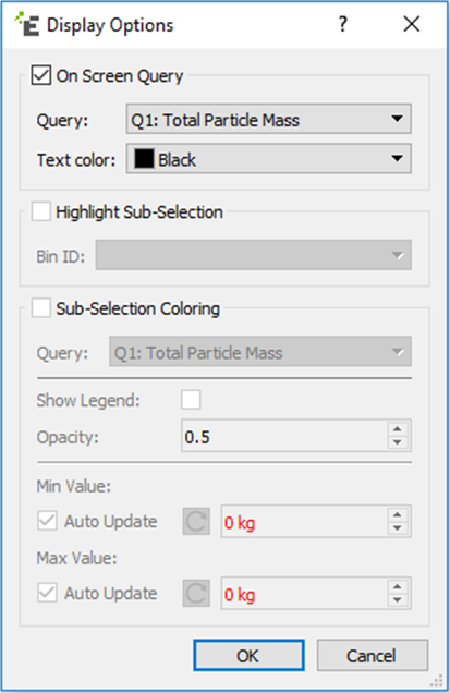
- Click the icon to view the results in real time.
As the playback continues through the Time Steps, bin group data is collected and displayed.
Plot Graphs
The last step in this tutorial is to learn to plot the data collected during your simulation using graphs.
-
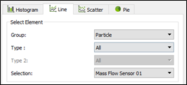
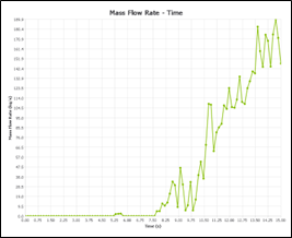
Plot a linear graph of mass flow rate of all particles changing over time on
the bottom conveyor.
- Click the
 icon on the toolbar. Note: If you cannot see this icon on your toolbar, expand the Standard toolbar.
 - Select the Line tab and set the parameters as follows:
- In the X-axis tab, ensure that the Time Range covers the whole simulation time.
- In the Y-axis tab, set the Primary Attribute to Mass Flow Rate.
- Click Create Graph to plot the graph.
- Click the
-
Plot the increase in mass over time and total particle mass in the rock
box.
The bin group over the rock box registers the change of total mass of the particles there.
- In the Line tab, set the parameters as follows:
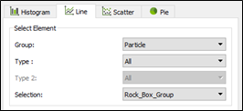
- In the X-axis tab, ensure that the Time Range covers the whole simulation time.
- In the Y-axis tab, set the Primary Attribute to Mass and the Component to Total.
- Click Create Graph to plot the graph.
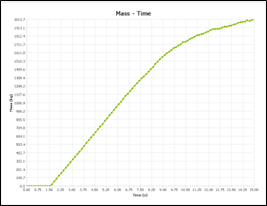
Note: From the graph, you can conclude that a steady state has not yet been reached.
- In the Line tab, set the parameters as follows: