EDEM Analyst - Analyze Your Results
Learn how to review, examine, and analyze the results of the simulation using EDEM Analyst.
-
Click the
 icon
on the Toolbar.
icon
on the Toolbar.
-
Use the controls
 below the simulation window to rewind the simulation to the first Time
Step.
below the simulation window to rewind the simulation to the first Time
Step.
-
Click the
 icon to play through each Time Step of your simulation.
Configure the Display
You can use the Display section in the Analyst Tree to configure the appearance of the different elements in your model. The Geometry, particles, and contacts within your model can also be colored in a variety of ways. Any section of a Geometry, particle, contact type, or selection group can be colored independently.
-
Configure the Geometries subsection.
Note: Geometry sections can be displayed as solid shapes, as meshes or as points (based on the mesh nodes). The opacity can also be altered. These display options can be applied to all of your geometry, or just to individual sections.
- Click Display in the Analyst Tree and then expand the Geometries subsection.
- Select different Geometries and modify their display in the Detailed View.
- Ensure that the Display Factory checkbox is not selected, so that it is not visible in the Viewer Window.
- Ensure that the Hopper is drawn as a Mesh and the screw blade is displayed as Filled with 0.7 opacity.
- Ensure that the factory plate Display checkbox is cleared.
-
Configure the Particles subsection.
You can modify the display of the particles in a similar way as that of the Geometries. In addition, you can represent the particles using cones, streams, and vectors that trace the direction in which the particles move.
- Click the
 icon to restart the simulation.
 - Select the Grain particle subsection in the
Analyst Tree.Note: To be able to view this section, at least some particles must be generated in the domain. Click the
 icon and the Grain particle should now
be available.
icon and the Grain particle should now
be available. - Set the Representation type to Vector.
- Click the icon to view how the direction of movement
of the particle changes over time.
- Click the
 icon at any point and set the
Representation type back to
Default.
icon at any point and set the
Representation type back to
Default.
- Click the
-
Configure the Contacts subsection.
You can select to show all contacts or only a subset of them. For example, just contacts between particles, or between particles and a particular section of geometry. You can display the contacts in a number of ways by using the contact vector, tangential force, normal force or normal overlap.
- Select Contact in the Analyst tree.
- Toggle the display of contacts between elements of different types.Note: It is recommended to temporarily turn off the display of particles for a clear view of the contacts.
- Before you finish, clear the Display Contacts checkbox and ensure that the particles Display is enabled.
-
Color the Geometries.
- Color the screw blade separately from the rest of the Geometry to highlight it.
- Select the screw blade Geometry element in the Analyst Tree.
- In the Coloring section of the Detailed View, select Uniform in the Color by dropdown list.
- Set the Color to the Dark Red to color the blade.
- Set the Color of the remaining sections of the Geometry to Dark Gray.
-
Color the particles according to their velocity.
- Select Grain particle in the Particles subsection of the Analyst Tree.
- In the Coloring section of the Detailed View, select Velocity in the Color by dropdown list.
- Select 3 levels of coloring and set the Min, Mid, and Max colors to Blue, Green, and Red respectively.
- Ensure that the Smooth Colors checkbox is cleared.
- Click next to the Min Value and Max Value fields to read the current values from the point in the simulation displayed in the Viewer.
- Select the Auto Update checkbox so that the values continue to update while the simulation is being played.
- Rewind the simulation back to the start and click the icon to view how the colors are updated as
the simulation progresses.
Extract Data
The next step is to export the data collected during your simulation for analysis. The data can be exported from a single Time Step, a range of Time Steps, all the elements in a model, or a selection or bin group.
-
Create an export configuration.
- Navigate to .
The Export Results Data dialog box is displayed.
- Click the
 icon below Configuration
ID to create a new configuration.
icon below Configuration
ID to create a new configuration. A single configuration can contain multiple queries that you can reuse at any point in your model.
- Set the Export format to Text to extract data to
a
.csvfile. - Enter the file name as Screw Auger and then
navigate to the save location which is the
tutorialfolder.
- Navigate to .
-
Define a query to export queries for each bin group.
Note: Since data has been saved every 0.01 s, exporting a large amount of data can cause a delay. In this lesson, the Export Data dialog box can be set to only export data every 0.1 s.
- Navigate to , and select the General tab.
- Select the Output Averages, Maximums, Minimums, and Totals in Columns checkbox.
- In the Time Steps section, clear the All checkbox and then set the Start time to 0 s and End time to ~10 s.
- In the Step Factor section, select Time and set the value to 0.1 s.
-
Select the Queries tab to define the data to be exported.
- Click the icon to create a new query.
- Name the query Velocity Query, by clicking the
 icon.
icon. - Click Particle and then select the Velocity attribute.
- Select Magnitude from the Component dropdown list.
- Select Average from the Query Type dropdown list.
- Ensure that the other options have their default settings.
- Click the
-
Add a query to export the X, Y and Z-position of each particle.
- Click the icon to create a second query and name it
Position Query X.
- Click Particle and then select the Position attribute.
- Select Average from the Component dropdown list.
- Select Average from the Query
Type dropdown list.
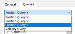
- Click the icon
 to copy the query and rename it to
Position Query Y.
to copy the query and rename it to
Position Query Y. - Select Y from the Component dropdown list.
- Repeat the same steps for the Z component.
- Click the
-
Export the data.
- Click Export to export the data to the pre-defined file.
- Open the file in an external application (such as a spreadsheet) and review the data.
Create a Video
EDEM allows you to export videos in AVI, WMV, MKV, MP4, WebM, or EnSight video file formats.
-
Set the video options.
- Click the
 in the Viewer. to record the animation.
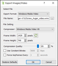
- In the Export Video dialog box, select Windows Media Video as the Export Format.
- Specify the file name and select a location to save the video.
For example save the file as
C:\EDEM_Tutorials\Screw_Auger_video.wmv - Select Windows Media Video V8 or any available
compressor.
EDEM will detect the compressor installed on your local machine and may vary depending on computer specifications.
- Click the
 icon to set the frame width and height to
be the same as the dimensions of the Viewer.
icon to set the frame width and height to
be the same as the dimensions of the Viewer. - Click OK. The record video icon changes to
 while recording.
- Click the
-
Record the video.
- Use the animation controls to play or step through the simulation.
- Click the , if necessary, and then click the icon.
- Experiment with stopping the playback, changing the camera angles and display options, and then restart playback.
- Once playback completes, click the icon again to save the video file.
- Open the video using Windows Media Player or any other media player.