Inputs
Introduction
The total number of user inputs is equal to 14.
Among these inputs, 4 are standard inputs and 10 are advanced inputs.
The maximum line current, the maximum Line-Line voltage and the rated power supply frequency allows to define the base speed point and in addition, the maximum speed allows to define the maximum speed point.
Standard inputs
- Maximum Line-Line voltage, rmsThe rms value of the maximum Line-Line voltage supplying the machine: “Maximum Line-Line voltage, rms” (Maximum Line-Line voltage, rms value) must be provided.Note: The number of parallel paths and the winding connection are automatically considered in the results.
- Rated power supply frequency
The value of the rated power supply frequency of the machine: “Rated power supply frequency” (rated power supply frequency) must be provided.
The rated power supply frequency is the electrical frequency applied at the terminals of the machine for the base speed point.
- Current definition mode There are three common ways to define the electrical current:
- Electrical current can be defined by the current density in electric conductors.
- Electric current can be defined directly by indicating the value of the maximum line current (the rms value is required).
- Electric current can be defined by a rated slip ratio which leads to impose a value of current (between the break down torque and zero torque).
The electrical current addition to the maximum Line-Line voltage and the rated power supply frequency allows to define the base speed point.
- Maximum line current, rms
The value of the maximum line current supplied to the machine “Maximum line current, rms” (Maximum line current, rms) must be provided. The maximum line current value corresponds to the line current targeted at the base speed point.
If you don’t know the value of “Maximum line current, rms”, the following identification process of the “Maximum line current, rms” at the “Base speed point” is recommended:- Solve the test “Characterization – Model – Motor – Scalar” (with the same inputs and settings are those to be applied for the test “Performance mapping – Sine wave – Motor – Efficiency map scalar).
- From the “Mechanical torque versus speed” curve, select the “Rated
power supply frequency value” (Yellow box on the following picture),
and the “Max. Line-Line voltage value” (Red box on the following
picture)
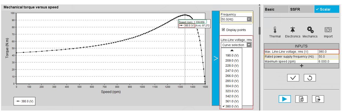
“Mechanical torque versus speed” curve, selection of the “Rated power supply frequency value” - Identify the speed at the break down torque (Green box on the previous picture)
-
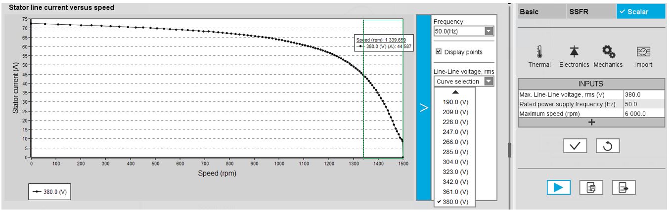
Following the previous steps, select the maximum current value you want to target at the base speed point.
The value of current selected must be between the speed at break down torque and the maximum speed (green box on the next picture)
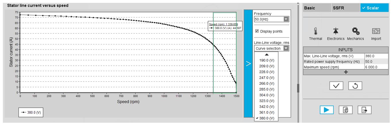
From the “Stator line current versus speed” curve, selection of the maximum current value Note:- The number of parallel paths and the winding connections are automatically considered in the results.
- The base speed point is also defined by the maximum line-line voltage and the rated power supply frequency.
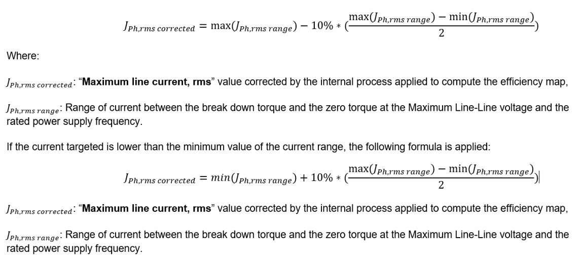
- In case the “Maximum line current, rms” set in input is higher or lower than those in the range defined by the break down torque and the zero torque, an automatic correction is done to target a realistic value (inside the range).
- Maximum current density, rms
The value of the rated current density in electric conductors “Max. current density, rms” (Maximum current density in conductors, rms) must be provided. The rated current density value corresponds to the current density targeted at the base speed point.
If the value of “Maximum current density, rms” is unknown, the following identification process of the “Maximum current density, rms” at the “Base speed point” is recommended:
- Solve the test “Characterization – Model – Motor – Scalar” (with the same inputs and settings are those to be applied for the test “Performance mapping – Sine wave – Motor – Efficiency map scalar”.
- From the “Mechanical torque versus speed” curve, select the “Rated power
supply frequency value” (Yellow box on the following picture) and the
“Max. Line-Line voltage value” (Red box on the following picture)
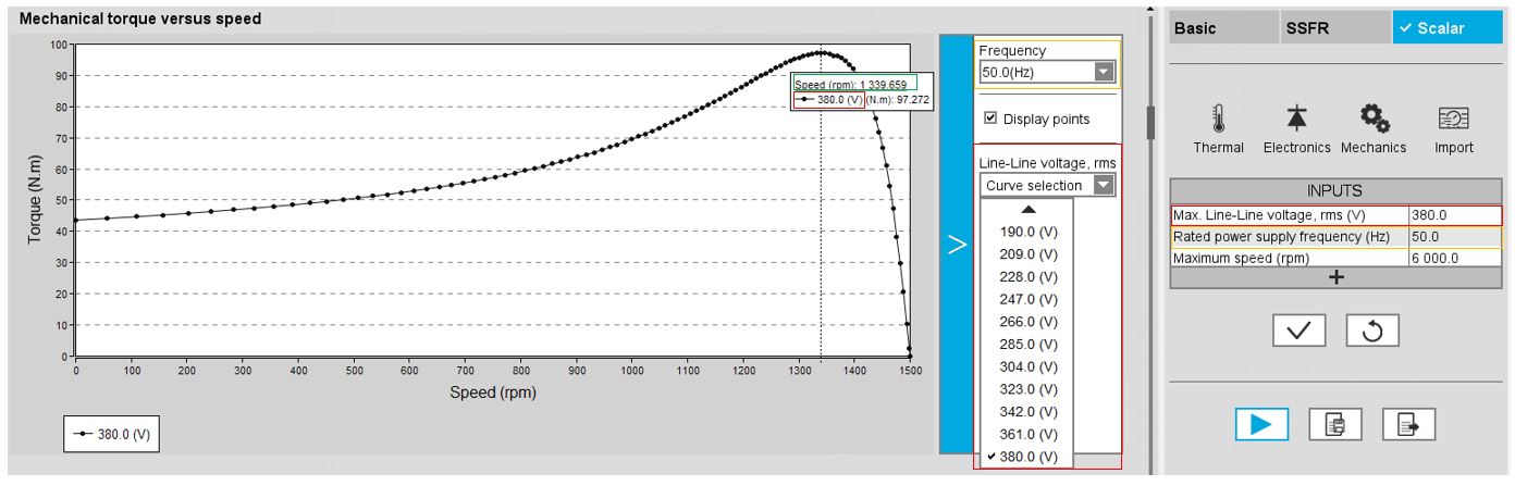
From the “Mechanical torque versus speed” curve, selection of the rated power supply frequency value - Identify the speed at the break down torque (Green box on the previous picture)
-
Following the previous steps, select the maximum current value you want to target at the base speed point.
The value of current selected must be between the speed at break down torque and the maximum speed (green box on the next picture).
From the “Stator line current versus speed” curve, selection of the maximum current value - By using the “Line current, rms” deduced, and finally the corresponding
“Current density, rms” can be computed using the following
formula:
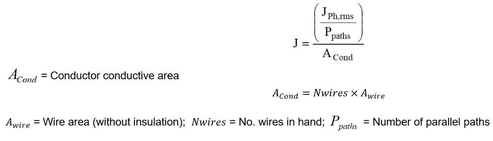
Note:- The number of parallel paths and the winding connections are automatically considered in the results.
- The base speed point is also defined by the maximum line-line voltage and the rated power supply frequency.
- In case the “Maximum current density, rms” set in input is
higher or lower than those in the range defined by the break
down torque and the zero torque, an automatic correction is
done to target a realistic value (inside the range).
- If the current density targeted is higher than the
value of the current density range, the following
formulas is applied:
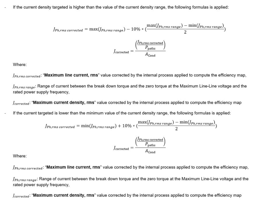
- If the current density targeted is higher than the
value of the current density range, the following
formulas is applied:
- Rated slip ratio
The value of the rated slip ratio of the machine “Rated slip ratio” (Rated slip ratio) must be provided.
The rated slip ratio corresponds to the ratio between the “slip (or speed) obtained from the targeted rated torque” and the “slip (or speed) range” (Slip range is defined between the break down torque and the zero torque).
The following picture describes the principle of computation.
This input allows the automatic computation of the related maximum line current at the base speed point.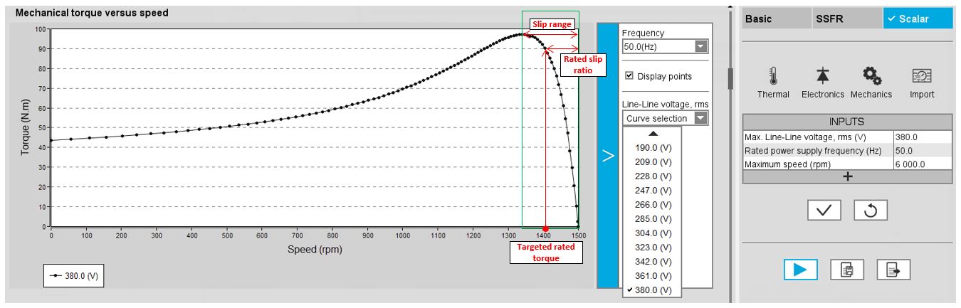
Torque vs speed curve - Rated slip ratio – Base speed point Note:- This way to target a maximum line current is the only one that is not subject to potential correction in function of the user value.
- The number of parallel paths and the winding connections are automatically considered in the results.
- The base speed point is also defined by the maximum line-line voltage and the rated power supply frequency.
- Maximum speed
The value of the « Maximum speed » (Maximum speed).) must be provided.
The analysis of test results is performed over a given speed range defined between 0 and the maximum speed. This allows the user to evaluate the behavior of the machine as a function of speed (like rotor Joule losses, total losses, power factor...) in this range.
Advanced inputs
- Electrical equivalent scheme identification
In the first step of the internal process of computation, it is needed to identify the model (non-linear electrical equivalent scheme – see “Characterization – Model – Motor – Scalar” for more details). That means computation for each component of the electrical scheme (resistance and inductances) maps in function of the Line-Line voltage and the power supply frequency.
The following inputs allow to fix the discretization required to identify the non-linear model.
- Model maps identification - Number of computations for Line-Line
voltage
The number of computations for the voltage must be defined with the user input « ID - No. Comp. for voltage » (Electrical equivalent scheme identification - Number of computations for Line-Line voltage).
The default value is equal to 10. This default value provides a good compromise between the accuracy and the computation time. The minimum allowed value is 10.Note: We recommend increasing « ID - No. Comp. for voltage » to at least 15 in case of fractional slot per pole and per phase. - Model maps identification - Number of computations for power supply
frequency
The number of computations for the frequency must be defined with the user input « ID - No. Comp. for freq. » (Electrical equivalent scheme identification - Number of computations for power supply frequency).
The default value is equal to 10. This default value provides a good compromise between the accuracy and the computation time. The minimum allowed value is 10.Note: We recommend increasing « ID - No. Comp. for freq. » to at least 15 in case of fractional slot per pole and per phase. - Operation of the non-linear model to generate
T(U,f,s)
In the second step of the internal process of computation, it is needed to operate (solve) the model (non-linear electrical equivalent scheme) to generate sets of curves in function of the Line-Line voltage, the power supply frequency, and the slip to get the performances of the machine as in the T(Slip) test.
Forth following inputs allow to fix the discretization required to operate the non-linear model in order to get the data set of T(U,f,s) curves representing the behavior of the machine in function of the Line-Line voltage, the power supply frequency and the slip (or speed).
- Operation of model to generate T(U,f,s) - Number of computations for
Line-Line voltage
The number of computations for the voltage must be defined with the user input « OP. - No. comp. for voltage » (Operation of model to generate T(U,f,s) - Number of computations for Line-Line voltage).
The default value is equal to 20. This default value provides a good overview of the machine behavior. The minimum allowed value is 10.Note: Values higher than the default value can be used, particularly in the case where, at low speed, some points of the torque-speed curve are fixed at "0" while the torque at zero speed is different from "0". There is a lack of robustness in the first version of this test, but increasing the number of calculations is usually the solution. - Operation of model to generate T(U,f,s) - Number of computations for
power supply frequency
The number of computations for the frequency must be defined with the user input « Op. - No. comp. for freq. » (Operation of model to generate T(U,f,s) - Number of computations for power supply frequency).
The default value is equal to 30. This default value provides a good overview of the machine behavior. The minimum allowed value is 10.Note: Values higher than the default value can be used, particularly in the case where, at low speed, some points of the torque-speed curve are fixed at "0" while the torque at zero speed is different from "0". There is a lack of robustness of the first version of this test, but increasing the number of calculations is usually the solution. - Operation of model to generate T(U,f,s) – Slip distribution
modeThe computation of the test « Characterization – Model – Motor – Scalar » is performed by considering a distribution of computed points. The user’s input “Slip distribution mode” (Select the method for the distribution of computed points) gives three possibilities to the user:
- Slip distribution mode = Logarithmic
When “Logarithmic” is selected, the distribution of the computed points is automatically done. The number of computations to be done in the slip range must be set in the next field: “No. comp. in slip range”.
- Slip distribution mode = Linear
When “Linear” is selected, the distribution of the computed points is automatically done. The number of computations to be done in the slip range must be set in the next field: “No. comp. in slip range”.
- Slip distribution mode = Table
When “Table” is selected, the list of slips to be considered must be defined by using the field: “Slip table” and then clicking on the button “Set values”.
Two ways are possible to fill the table: either filling the table line by line or by importing an excel file, where all the slips to be considered are defined.Note: The slips must be listed in ascending order.
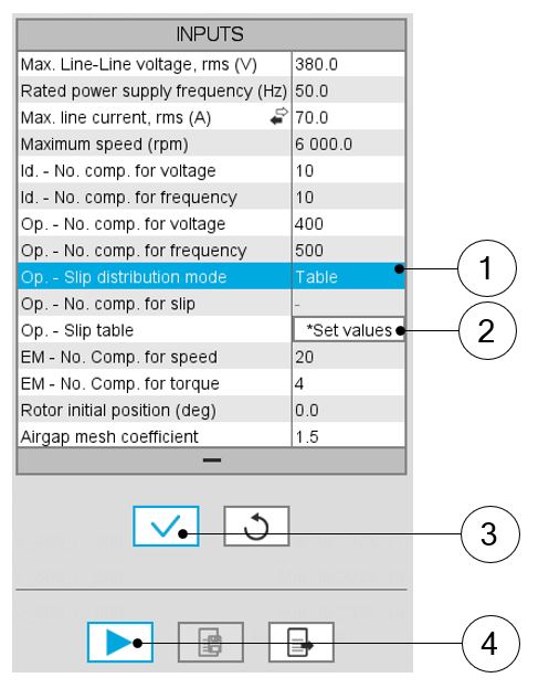
Slip distribution mode = Table 1 Select the “Table” option. 2 Click the button “Set values” of the field “Slip table” to open a dialog box defining the list of slips to be considered.
Refer to the next illustration which shows how to fill the Slip table.
3 Button to validate and consider the user inputs 4 Button to run the computation 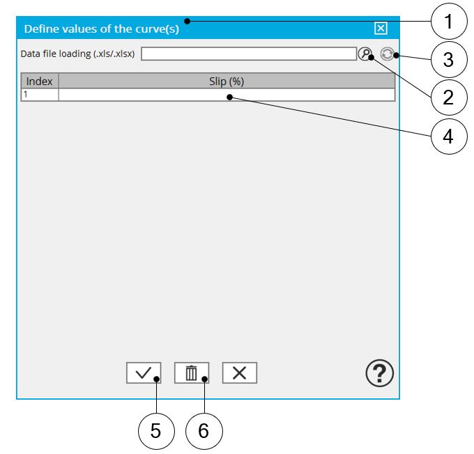
Slip distribution mode = Table – Dialog box to define the list of slips 1 Dialog box opened when clicking on the button “Set values” in the field “Slip table” 2 Browse the folder to select an Excel file which defines the list of slips 3 Button to refresh the table data when the considered Excel file has been modified 4 Fields to be filled with data to describe the considered slips 5 Button to apply the inputs 6 Button to erase the data table Note: The Excel template used to import the list of slips is stored in the folder Resource/Template in the installation folder of FluxMotor®. An example of this template is displayed below.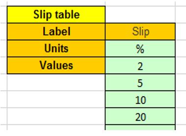
Excel file template to define the list of slips Note:- The slips must be listed in ascending order.
- We recommend to define at least 100 values to get an accuracy high enough, (especially since going below 100 does not lead to a significant reduction in computation time).
- Slip distribution mode = Logarithmic
- Operation of model to generate T(U,f,s) - Number of computations for
slip
The number of computations for the slip must be defined with the user input « Op. - No. comp. for slip » (Operation of model to generate T(U,f,s) - Number of computations for slip).
The default value is equal to 100. This default value provides a good overview of the machine behavior.
The minimum allowed value is 10 it is recommended not to go below 100 to get a high enough accuracy (especially since going below 100 does not lead to a significant reduction in computation time).Note:- The machine operating mode is “Motor”, so the slip range is [0,1].
- The slip distribution mode used is logarithmic or linear.
- The computation time of the test is not highly impacted by this input and huge values such as 200 can be used.
- Operation of model to generate T(U,f,s) – Slip
tableWhen the choice of point distribution mode is “Table”, the list of slips to be considered “Op. - Slip table” (Operation of model to generate T(U,f,s) - Slip table) must be provided. Refer to the above section 2) Slip distribution mode = TableNote: The machine operating mode is fixed to “Motor”, so the slip range is ]0,1].
- Efficiency map computation parameters
As a final step of the internal process of computation, it is needed to apply the scalar command.
The command is applied to the data set generated in the previous step (Operation of model to generate T(U,f,s)) through an automatic post-processing.
With this post-processing the behavior of the machine in the torque speed plane is obtained in consistency with the scalar command.
The following inputs allow to fix the discretization required to compute the efficiency map and associated results in the torque-speed plane.
- EM - Number of computations for speed
The “EM - No. comp. for speed” (Efficiency map - Number of computations for speed) corresponds to the number of points to be considered in the speed range from 0 to the maximum speed.
Half of these points are distributed from 0 to the base speed. The remaining points are distributed from the base speed to the maximum speed.
In both cases, base speed is considered as an additional point.
Note: If the user input parameter “No. comp. for speed” is an odd number, one discretization point is automatically removed.
The default value is equal to 20. The minimum allowed value is 10 while the maximum recommended value is 40.Note: Increasing the number of computations can improve the convergence of the optimization used to define the torque-speed curve and the efficiency map. However, that also means longer computation time. - EM - Number of computations for torque
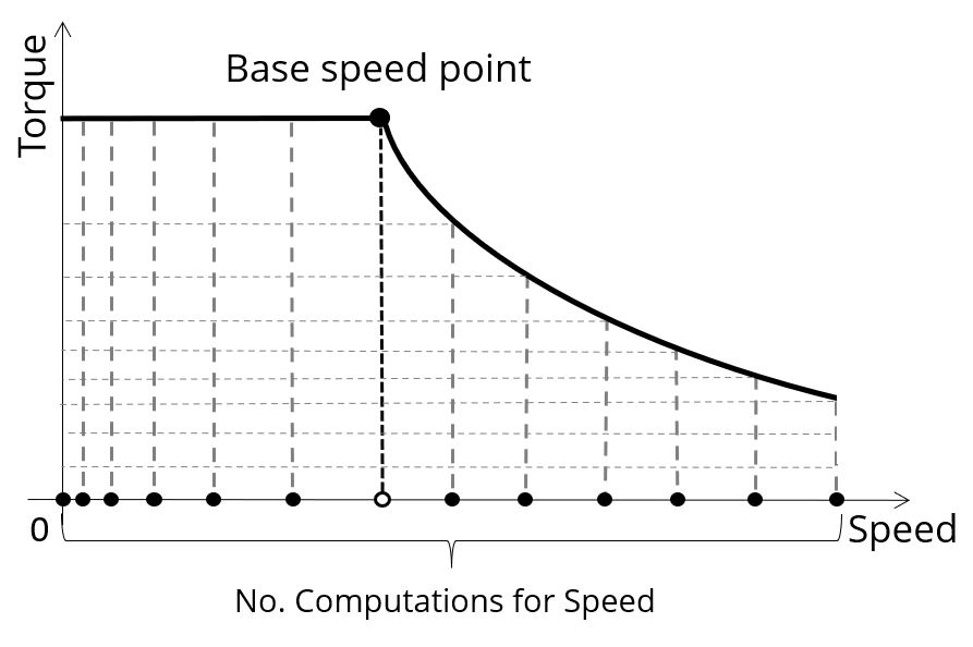
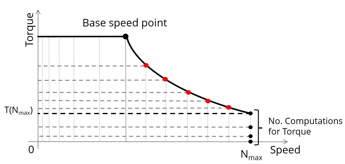
For the speed range [Nbase; Nmax.], the number of computations for torque is imposed by the number of computations for the defined speed range [Nbase; Nmax.] (Red points in the image shown below).
The advanced user input parameter “EM - No. comp. for torque” (Efficiency map - Number of computations for torque) allows to finalize the grid within the torque range [0, T (Nmax.)] at the maximum speed (Black points in the image shown below).
The default value is equal to 4. The minimum allowed value is 4 while the maximum recommended value is 10.
- Skew model – No. of layers
When the rotor bars or the stator slots are skewed, the number of layers used in Flux® Skew environment to model the machine can be modified: “Skew model - No. of layers” (Number of layers for modelling the skewing in Flux® Skew environment).
- Rotor initial position
The initial position of the rotor considered for computation can be set by the user in the field « Rotor initial position » (Rotor initial position). The default value is equal to 0.
The range of possible values is [-360, 360].
The rotor initial position has an impact only on the induction curve in the air gap.
- Airgap mesh coefficient
The advanced user input “Airgap mesh coefficient” is a coefficient which adjusts the size of mesh elements inside the airgap. When the value of “Airgap mesh coefficient” decreases, the mesh elements get smaller, leading to a higher mesh density inside the airgap, thereby increasing the computation accuracy.
The imposed Mesh Point (size of mesh elements touching points of the geometry), inside the Flux® software, is described as:
MeshPoint = (airgap) x (airgap mesh coefficient)
Airgap mesh coefficient is set to 1.5 by default.
The variation range of values for this parameter is [0.05; 2].
0.05 gives a very high mesh density and 2 gives a very coarse mesh density.CAUTION:Be aware, a very high mesh density does not always mean a better result quality. However, this always leads to a huge number of nodes in the corresponding finite element model. So, it means a need of huge numerical memory and increases the computation time considerably.