Urban Dominant Path Model
The dominant path model (DPM) determines exactly this dominant path between the transmitter and each receiver pixel. The computation time compared to ray-tracing is significantly reduced and the accuracy is nearly identical to ray-tracing.
Ray-optical propagation models are still very time-consuming – even with accelerations like preprocessing. And what is even more important, they rely on a very accurate vector database. Small errors in the database influence the accuracy of the prediction. On the other hand, empirical models rely on dedicated propagation effects like the over-rooftop propagation (for example the direct ray COST 231). A comparison of prediction results computed with three types of prediction models is presented in the following figure.
Analyzing typical propagation scenarios shows that in most cases one propagation path contributes more than 90% of the total energy. The dominant path model (DPM) determines exactly this dominant path between the transmitter and each receiver pixel. So the computation time compared to ray-tracing is significantly reduced and the accuracy is nearly identical to ray-tracing.
Empirical models (like COST 231) consider only the direct path between a transmitter and a receiver pixel. Ray tracing models (like IRT) determine numerous paths. DPM determines only the most relevant path, which leads to short computation times.
Advantages of the Dominant Path Model
- The dependency on the accuracy of the vector database is reduced (compared to ray-tracing).
- Only the most important propagation path is considered, because this path delivers the main part of the energy.
- No time-consuming preprocessing is required (in contrast to IRT).
- Short computation time.
- Accuracy reaches or exceeds the accuracy of ray-optical models.
Typical Application of the Dominant Path Model
As the dominant path model does not require a preprocessing of the vector building database it is ideally suited for very large areas. Additionally the approach to compute only the dominate ray emphasizes this operational area. The model does not compute the complete channel impulse response, thus if the user is interested in the channel impulse response, the delay spread or the angular spread, a ray-tracing model is recommended. The DPM is the ideal approach to compute coverage predictions in large urban areas.
Algorithm of the Dominant Path Model
The DPM determines the dominant path between transmitter and each receiver pixel. The computation of the path loss is based on the following equation:
- Distance from transmitter to receiver ( )
- Path loss exponent ( )
- Wave length ( )
- Individual interaction losses due to diffractions ( )
- Empirically determined loss reduction due to wave guiding ( )
- Gain of transmitting antenna ( )
As described above, is length of the path between transmitter and current receiver location. p is the path loss exponent. The value of depends on the current propagation situation. In dense urban areas p tends to be slightly higher than in open areas. See Table 1 for further guidance. In addition, p depends on the breakpoint distance. After the breakpoint, increased path loss exponents are common due to distortions of the propagating wave. The function yields the loss (in dB) which is caused by diffractions. The diffraction losses are accumulated along one propagation path. Reflections and scattering are included empirically. For the consideration of reflections (and scattering), an empirically determined wave guiding factor is introduced. This wave guiding factor takes into account, that a wave propagating in a long street canyon will be reflected on the walls leading to less attenuation compared to free space. Thus, wave guiding effects can be expressed as an additional gain in dB. The directional gain of the antenna (in direction of the propagation path) is also considered.
Configuration of the Dominant Path Model
The following screenshot shows the configuration dialog of the DPM.
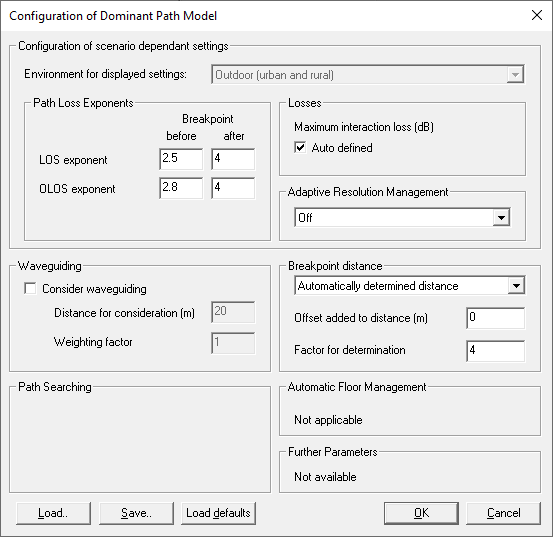
- Path Loss Exponents
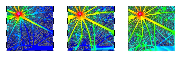
- The path loss exponents influence the propagation result computed by the DPM significantly. The path loss exponents describe the attenuation with distance. A higher path loss exponent leads to a higher attenuation in same distance. The following figure shows a comparison of three predictions with different path loss values for the LOS area.
-
Figure 5. Path loss predictions based on three different path loss values. LOS exponent 2.0 (on the left), LOS exponent 2.3 (middle) and LOS exponent 2.6 (to the right). 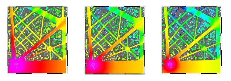
The following table shows recommended path loss exponents, depending on the height of the transmitter. The density of obstacles in the real scenario which are not modeled in the vector database do also influence the path loss exponent. The more objects that are missing in the vector database, the higher the path loss exponent should be.
- Interaction losses
- Each change in the direction of propagation due to an interaction (diffraction, transmission / penetration) along a propagation path causes an additional attenuation. The maximum attenuation can be defined. The effective interaction loss depends on the angle of the diffraction. It is recommended to select Auto. The transmitter frequency will then be taken into account in the calculation of maximum interaction loss.
- Waveguiding effects
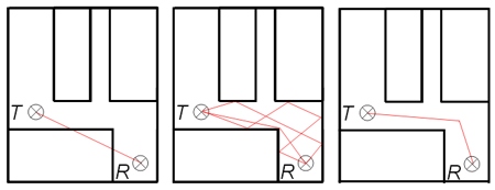
- As mentioned before, the DPM includes wave guiding effects to achieve highly accurate results. Two parameters are available to configure the wave guiding module. The first parameter is used to define the maximum distance to walls to be included in the determination of the wave guiding factor. With the second parameter the weight of the wave guiding effects in the computation of the path loss is defined (1.0 is suggested. Values below 1.0 reduce the influence of the wave guiding factor and values above 1.0 increase it). In typical scenarios the wave guiding effects can be turned off, this reduces the prediction time
- Adaptive resolution management
-
For acceleration purposes, the DPM offers an adaptive resolution. In close streets a fine resolution is used for the prediction and on large places or open areas DPM switches automatically to a coarse resolution. The prediction time and the memory demand are positively influenced by the adaptive resolution but the accuracy is limited - especially if the highest level for the adaptive resolution is selected by the user.
For the adaptive resolution management, the level (factor) can be specified. Possible levels (factors) are 0, 1, 2, 3, and 4. Level 0 disables the adaptive resolution management (each pixel is computed with the DPM algorithm).
As the level is increased, fewer and fewer pixels are computed in open areas (for example, for Level 1 every other pixel is computed) and the remaining ones are interpolated. The adaptive resolution management is not applied close to the transmitter.- Factor 1 is only applied for distances larger than 400m.
- Factor 2 is only applied for distances larger than 800m.
- Factor 3 is only applied for distances larger than 1000m.
- Factor 4 is only applied for distances larger than 1200m.
Additional Features
- Consideration of vegetation in urban environment
- Vegetation databases describe areas of vegetation with polygonal cylinders (individual height for each cylinder possible). Additional attenuation can be defined for each vegetation element. All paths penetrating the vegetation get an additional loss per meter (in dB/m) and all signals at receiver locations inside the vegetation blocks are additionally attenuated (loss in dB). This makes sure that the prediction result is not too optimistic, if dense vegetation is present. Vegetation databases describe areas of vegetation with polygonal cylinders (individual height for each cylinder possible). Additional attenuation can be defined for each vegetation element. All paths penetrating the vegetation get an additional loss per meter (in dB/m) and all signals at receiver locations inside the vegetation blocks are additionally attenuated (loss in dB). This makes sure that the prediction result is not too optimistic, if dense vegetation is present.
- Combined network planning
- The DPM offers the CNP mode which allows the combination of urban and indoor predictions. In the urban environment the prediction is computed with the urban dominant path model (UDP), its settings and the resolution selected for the urban domain. For the predictions in the indoor area the indoor dominant path model (IDP) with a higher resolution is used. The settings of the dominant path model, such as path loss exponents and interaction losses, can be defined for both environments (urban and indoor) individually.
Auto Calibration
The model can be calibrated automatically.