Reduce Computation Time for Large Databases
For large databases, computation time can be reduced by defining database areas where ray interactions are tracked.
Even then, depending on the simulation method, simulation times can be long because the tool still investigates how interactions of rays with all buildings (including those far away) affect the results in the prediction area. To reduce the simulation time further, you can define a polygon that describes which database area is to be included in the tracking of the ray interactions.
Create the polygons by clicking or use the ![]() icon.
icon.
Since the database area applies to vector objects, it is available in indoor and urban scenarios, including scenarios with vector topography (ground described by triangles, for example, via a file with .tdv extension). It is not available in rural scenarios based on pixel databases (files with .tdb extension).
As for time-variant scenarios, any database area is active for all time steps but the polygons (the geometry selection) can only be drawn with the first time step and this selection is the same for all the time steps.
To manage all the database areas open the Database Polygons dialog. Click . Select the Building Data tab and under Database Polygons, select the Consider database polygons check box and click Settings to launch the Database Polygons dialog.
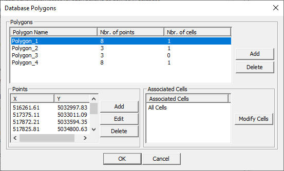
- Add a new polygon.
- Delete an existing polygon.
- Add a new point to a polygon. The position of the point can be specified by selecting one of the existing points (the position will be next the selected point), if no position was specified the point will be added to the end of the points list.
- Edit an existing point.
- Delete an existing point.
- When adding, editing, or deleting a point, some checks are performed if the polygon is still valid (does not intersect itself and it has at least three points).
- Modify the assigned transmitters to this polygon.
- If a cell does not have a polygon, the whole database is considered as usual.
- If a cell has one or more polygons, the objects that are inside any one of the polygons are considered while the remaining objects are ignored.
In case of vector topography, the selection of database area also applies to the triangles that represent the ground. In that case, it is important to choose the database area large enough to include the entire prediction area, otherwise the topo height at some prediction pixels is no longer properly defined.
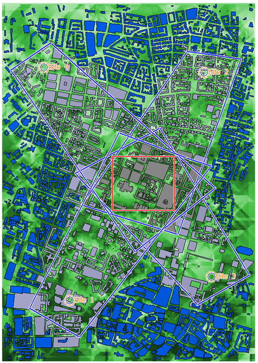
If you have multiple transmitters and a modest prediction area between them, defining database areas (see Figure 5) can be efficient. The prediction area (the red rectangle where results is computed) is part of all database areas, and each individual database area also includes the buildings between the transmitter and the prediction area.
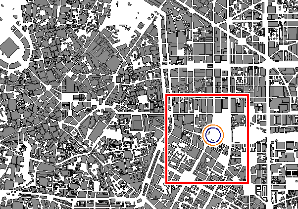
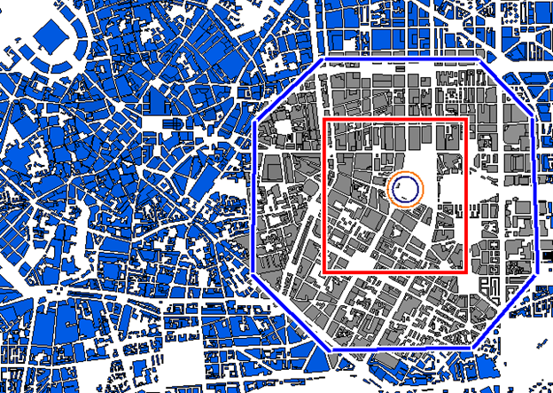
- The objects, which are ignored by all transmitters, are considered as virtual objects and are represented in blue.
- The objects, which are considered by all the transmitters, are represented by its default color.
- The objects, which are considered by one ore more transmitters and ignored by other transmitters, are considered as partially virtual and are represented in light blue.